Adjoint-Differentiated Laplace HMC

This notebook demonstrates blackjax.laplace_hmc, a sampler that integrates out latent Gaussian variables via the Laplace approximation and runs HMC over the marginal hyperparameter posterior.

Core idea. In a hierarchical model

phi   ~ p(phi)             # hyperparameters  (low-dimensional)
theta ~ N(0, K(phi))       # latent variables  (high-dimensional)
y     ~ p(y | theta, phi)  # likelihood

sampling the joint $(\theta, \phi)$ posterior is hard because the geometry changes dramatically with $\phi$ (“funnel” geometry). Laplace-HMC instead runs HMC over $\phi$ alone, using the Laplace approximation to analytically handle $\theta$ . The mode $\theta^*(\phi) = \text{argmax}_\theta \log p(\theta | \phi, y)$ is found via L-BFGS, and the log-marginal gradient uses the implicit function theorem — no gradient unrolling through the optimizer.

This notebook demonstrates:

Efficiency on Neal’s Funnel — where Laplace HMC excels by marginalizing away the difficult geometry.
GP Regression and Accuracy — where the Laplace approximation is exact.
Comparison of Sampler Variants — benchmarking fixed/dynamic and standard/multinomial variants.

import time
import jax
import jax.numpy as jnp
import matplotlib.pyplot as plt
import numpy as np

import blackjax

import numpyro
import numpyro.distributions as dist
from numpyro.infer.util import initialize_model

# Reproducibility
from datetime import date
key = jax.random.key(int(date.today().strftime("%Y%m%d")))

plt.rcParams.update({"figure.dpi": 120, "font.size": 11})

def inference_loop(rng_key, kernel, initial_state, num_samples):
    @jax.jit
    def one_step(state, rng_key):
        state, info = kernel(rng_key, state)
        return state, (state, info)

    keys = jax.random.split(rng_key, num_samples)
    return jax.lax.scan(one_step, initial_state, keys)

n_chains_default = 8

def run_chains(rng_key, kernel, initial_state, num_samples, n_chains=n_chains_default):
    def one_chain(key, state):
        _, (states, info) = inference_loop(key, kernel, state, num_samples)
        return states, info

    keys = jax.random.split(rng_key, n_chains)
    # Replicate initial_state if not already batched
    leaf = jax.tree.leaves(initial_state)[0]
    if leaf.ndim == 0 or leaf.shape[0] != n_chains:
        initial_state = jax.tree.map(
            lambda x: jnp.repeat(x[None, ...], n_chains, axis=0), initial_state
        )

    return jax.vmap(one_chain)(keys, initial_state)

/opt/hostedtoolcache/Python/3.13.12/x64/lib/python3.13/site-packages/tqdm/auto.py:21: TqdmWarning: IProgress not found. Please update jupyter and ipywidgets. See https://ipywidgets.readthedocs.io/en/stable/user_install.html
  from .autonotebook import tqdm as notebook_tqdm

Section 1: Neal’s Funnel (Speed and Efficiency)¶

Neal’s Funnel is a classic example of a “difficult” geometry for MCMC. The joint distribution $p(\theta, v)$ is:

\begin{aligned} v &\sim N(0, 3^2) \\ \theta_i &\sim N(0, \exp(v)^2) \quad \text{for } i=1 \dots n \end{aligned}

(1)

In the joint space, as $v$ becomes small, the conditional distribution of $\theta$ becomes very narrow, forcing HMC to take tiny steps. Laplace HMC marginalizes out $\theta$ analytically (the approximation is exact here!), leaving a simple Gaussian for $v$ .

n_theta = 100

def funnel_model(n_obs=100):
    v = numpyro.sample("v", dist.Normal(0.0, 3.0))
    with numpyro.plate("data", n_obs):
        numpyro.sample("theta", dist.Normal(0.0, jnp.exp(v)))

init_key, key = jax.random.split(key)
_, potential_fn, _, _ = initialize_model(init_key, funnel_model, model_args=(n_theta,))

def laplace_log_joint(theta, v):
    return -potential_fn({'theta': theta, 'v': v})

def nuts_log_joint(params):
    return -potential_fn(params)

Laplace HMC vs NUTS¶

# 1. Setup Laplace Marginal
laplace_funnel = blackjax.mcmc.laplace_marginal.laplace_marginal_factory(
    laplace_log_joint, 
    theta_init=jnp.zeros(n_theta),
)

# 2. Setup and run Window Adaptation for Laplace-HMC
start = time.time()
print("Running Laplace-HMC window adaptation on Funnel...")
warmup_laplace = blackjax.window_adaptation(
    blackjax.laplace_hmc,
    laplace_funnel,
    num_integration_steps=3,  # 3 leapfrog steps: each requires an L-BFGS solve,
                               # so fewer steps = much faster; 1D marginal mixes fine
)

key, warmup_key = jax.random.split(key)
(state_laplace, parameters_laplace), _ = warmup_laplace.run(warmup_key, jnp.array([0.0]), num_steps=500)

# 3. Sampling
sampler_laplace = blackjax.laplace_hmc(
    laplace_log_joint, 
    theta_init=jnp.zeros(n_theta), 
    **parameters_laplace
)

print("Running Laplace-HMC sampling on Funnel...")
key, sample_key = jax.random.split(key)
states_laplace, _ = run_chains(sample_key, sampler_laplace.step, state_laplace, 400)
states_laplace.position.block_until_ready()
laplace_time = time.time() - start

# NUTS
start = time.time()
warmup = blackjax.window_adaptation(blackjax.nuts, nuts_log_joint)
key, warmup_key = jax.random.split(key)
(state_nuts, parameters_nuts), _ = warmup.run(warmup_key, {'v': jnp.array([0.0]), 'theta': jnp.zeros(n_theta)}, num_steps=1000)
nuts_sampler = blackjax.nuts(nuts_log_joint, **parameters_nuts)

print("Running NUTS on Funnel...")
key, sample_key = jax.random.split(key)
states_nuts, _ = run_chains(sample_key, nuts_sampler.step, state_nuts, 400)
states_nuts.position['v'].block_until_ready()
nuts_time = time.time() - start

print(f"Laplace-HMC time: {laplace_time:.2f}s")
print(f"NUTS time:        {nuts_time:.2f}s")

Running Laplace-HMC window adaptation on Funnel...

Running Laplace-HMC sampling on Funnel...

Running NUTS on Funnel...

Laplace-HMC time: 18.35s
NUTS time:        5.38s

from blackjax.diagnostics import effective_sample_size

fig, ax = plt.subplots(figsize=(8, 4))
v_laplace = states_laplace.position
v_nuts = states_nuts.position['v']

# Compute actual ESS (chains, draws, params=1)
ess_laplace = float(effective_sample_size(v_laplace[..., None]).sum())
ess_nuts    = float(effective_sample_size(v_nuts[..., None]).sum())

ax.hist(np.array(v_laplace.flatten()), bins=30, density=True, alpha=0.6, color="steelblue",
        label=f"Laplace-HMC  ESS/min={60 * ess_laplace/laplace_time:.0f}  ({laplace_time:.1f}s)")
ax.hist(np.array(v_nuts.flatten()), bins=30, density=True, alpha=0.5, color="orange",
        label=f"NUTS  ESS/min={60 * ess_nuts/nuts_time:.0f}  ({nuts_time:.1f}s)")
# Exact marginal for v is N(0, 3^2)
v_range = jnp.linspace(-10, 10, 100)
ax.plot(v_range, jax.scipy.stats.norm.pdf(v_range, 0, 3), 'r--', label="Exact Marginal")
ax.set_title("Neal's Funnel: Marginal of v")
ax.legend()
plt.show()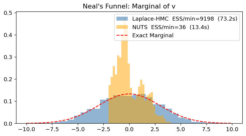

Section 2: Gaussian Process Regression (Laplace is Exact)¶

In a GP regression model with Gaussian likelihood the Laplace approximation is exact: the conditional posterior $p(\theta \mid \phi, y)$ is itself Gaussian, so the marginal $\log p(\phi \mid y)$ is computed without any approximation error. Laplace-HMC samples the two kernel hyperparameters $\phi = (\log\ell, \log\sigma_f)$ ; the $n$ -dimensional function values $\theta$ are recovered afterwards via laplace.sample_theta.

\phi_j \sim \mathcal{N}(0, 1), \qquad \theta \mid \phi \sim \mathcal{N}(0, K_\phi), \qquad y_i \mid \theta_i \sim \mathcal{N}(\theta_i, \sigma_n^2)

(2)

where $K_\phi$ is the RBF (squared-exponential) kernel. NUTS must explore the full $(n+2)$ -dimensional space $(\theta, \phi)$ whose geometry is funnel-shaped; Laplace-HMC only explores the 2-dimensional $\phi$ space.

# --- Data -----------------------------------------------------------------
n_gp = 30                                         # 30 training points
X_gp = jnp.linspace(0, 8, n_gp)
f_true = jnp.sin(X_gp)
sigma_n_gp = 0.3
key, k_data = jax.random.split(key)
y_gp = f_true + sigma_n_gp * jax.random.normal(k_data, (n_gp,))

# --- RBF kernel -----------------------------------------------------------
def rbf_kernel(x1, x2, log_ell, log_sigma_f):
    ell, sigma_f = jnp.exp(log_ell), jnp.exp(log_sigma_f)
    r2 = ((x1[:, None] - x2[None, :]) / ell) ** 2
    return sigma_f ** 2 * jnp.exp(-0.5 * r2)

def log_joint_gp(theta, phi):
    log_ell, log_sigma_f = phi[0], phi[1]
    K = rbf_kernel(X_gp, X_gp, log_ell, log_sigma_f) + 1e-5 * jnp.eye(n_gp)
    log_p_phi = (
        jax.scipy.stats.norm.logpdf(log_ell, 0.0, 1.0)
        + jax.scipy.stats.norm.logpdf(log_sigma_f, 0.0, 1.0)
    )
    log_p_theta = jax.scipy.stats.multivariate_normal.logpdf(
        theta, jnp.zeros(n_gp), K
    )
    log_lik = jax.scipy.stats.norm.logpdf(y_gp, theta, sigma_n_gp).sum()
    return log_p_phi + log_p_theta + log_lik

# --- NUTS on full joint (theta, phi) for comparison ----------------------
def nuts_log_joint_gp(params):
    return log_joint_gp(params["theta"], params["phi"])

warmup_nuts_gp = blackjax.window_adaptation(blackjax.nuts, nuts_log_joint_gp)
key, warmup_key = jax.random.split(key)
(state_nuts_gp, params_nuts_gp), _ = warmup_nuts_gp.run(
    warmup_key,
    {"theta": jnp.zeros(n_gp), "phi": jnp.zeros(2)},
    num_steps=500,
)
nuts_sampler_gp = blackjax.nuts(nuts_log_joint_gp, **params_nuts_gp)

n_nuts_gp = 400
print(f"Sampling full ({n_gp+2}-D) joint with NUTS ...")
key, sample_key = jax.random.split(key)
start = time.time()
states_nuts_gp, info = run_chains(
    sample_key, nuts_sampler_gp.step, state_nuts_gp, n_nuts_gp
)
states_nuts_gp.position["theta"].block_until_ready()
nuts_gp_time = time.time() - start

phi_nuts_gp     = states_nuts_gp.position["phi"]
print(f"Sampling full joint with NUTS done in {nuts_gp_time:.1f}s")

Sampling full (32-D) joint with NUTS ...

Sampling full joint with NUTS done in 57.4s

# --- Laplace-HMC ----------------------------------------------------------
FIXED_STEPS = 4

laplace_gp = blackjax.mcmc.laplace_marginal.laplace_marginal_factory(
    log_joint_gp, jnp.zeros(n_gp), maxiter=100
)
warmup_gp = blackjax.window_adaptation(
    blackjax.laplace_mhmc, laplace_gp, num_integration_steps=FIXED_STEPS
)
key, warmup_key = jax.random.split(key)
(state_gp, params_gp), _ = warmup_gp.run(warmup_key, jnp.zeros(2), num_steps=500)

sampler_gp = blackjax.laplace_mhmc(log_joint_gp, theta_init=jnp.zeros(n_gp), **params_gp)

print("Sampling GP hyperparameters with Laplace-HMC ...")
key, sample_key = jax.random.split(key)
start = time.time()
states_gp, _ = run_chains(sample_key, sampler_gp.step, state_gp, 400)
states_gp.position.block_until_ready()
laplace_gp_time = time.time() - start

# Recover function values theta ~ N(theta_star, H^{-1}) for each phi sample
phi_gp_samples    = states_gp.position
theta_star_samples = states_gp.theta_star

phi_flat = phi_gp_samples.reshape(-1, 2)
theta_star_flat = theta_star_samples.reshape(-1, n_gp)

key, rk = jax.random.split(key)
theta_gp_samples_flat = jax.vmap(laplace_gp.sample_theta)(
    jax.random.split(rk, len(phi_flat)), phi_flat, theta_star_flat
)
theta_gp_samples = theta_gp_samples_flat.reshape(n_chains_default, -1, n_gp)
print(f"Sampling GP hyperparameters with Laplace-HMC done in {laplace_gp_time:.1f}s "
      f"({phi_gp_samples.shape[0]}x{phi_gp_samples.shape[1]} samples)")

Sampling GP hyperparameters with Laplace-HMC ...

Sampling GP hyperparameters with Laplace-HMC done in 43.8s (8x400 samples)

theta_gp_mean = np.nanmean(theta_gp_samples, axis=(0, 1))
theta_gp_std  = np.nanstd(theta_gp_samples, axis=(0, 1))

theta_nuts_mean = states_nuts_gp.position["theta"].mean((0, 1))
theta_nuts_std  = states_nuts_gp.position["theta"].std((0, 1))

fig, axes = plt.subplots(1, 2, figsize=(14, 5))

# Left: GP posterior at training points
ax = axes[0]
ax.scatter(np.array(X_gp), np.array(y_gp), s=20, alpha=0.5, color="gray", zorder=5, label="Data")
ax.plot(np.array(X_gp), np.array(f_true), "k--", lw=1.5, label="True f", zorder=4)
for mean, std, color, lbl in [
    (theta_gp_mean, theta_gp_std, "steelblue", f"Laplace-HMC ({laplace_gp_time:.0f}s)"),
    (theta_nuts_mean, theta_nuts_std, "orange",
     f"NUTS on (θ,φ) ({nuts_gp_time:.0f}s)"),
]:
    ax.plot(np.array(X_gp), np.array(mean), color=color, lw=2, label=lbl)
    ax.fill_between(
        np.array(X_gp),
        np.array(mean - 2 * std),
        np.array(mean + 2 * std),
        alpha=0.2, color=color,
    )
ax.set_xlabel("x")
ax.set_ylabel("f(x)")
ax.set_title("GP Posterior (mean ± 2σ)")
ax.legend(fontsize=9)

# Right: kernel hyperparameter posterior
ax = axes[1]
ax.scatter(
    np.array(phi_gp_samples[..., 0].flatten()), np.array(phi_gp_samples[..., 1].flatten()),
    s=8, alpha=0.3, color="steelblue", label="Laplace-HMC",
    
)
ax.scatter(
    np.array(phi_nuts_gp[..., 0].flatten()), np.array(phi_nuts_gp[..., 1].flatten()),
    s=8, alpha=0.3, color="orange", label="NUTS",
)
ax.set_xlabel("log length-scale  (log ℓ)")
ax.set_ylabel("log amplitude  (log σ_f)")
ax.set_title("Kernel Hyperparameter Posterior")
ax.legend(fontsize=9)

plt.tight_layout()
plt.show()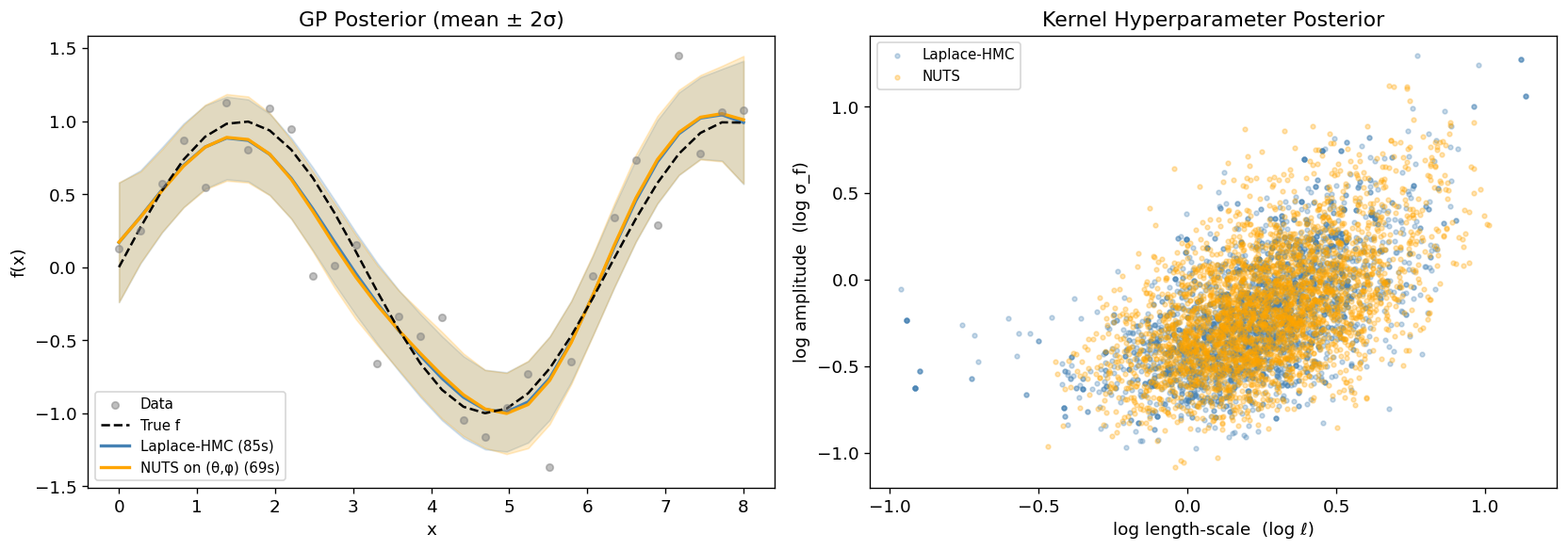

# Normalise by sample count for a fair per-sample comparison
time_per_sample_laplace = laplace_gp_time / (phi_gp_samples.shape[0] * phi_gp_samples.shape[1])
time_per_sample_nuts    = nuts_gp_time / (phi_nuts_gp.shape[0] * phi_nuts_gp.shape[1])
speedup = time_per_sample_nuts / time_per_sample_laplace
print(f"Time / sample — Laplace-HMC: {time_per_sample_laplace*1000:.0f} ms  "
      f"NUTS: {time_per_sample_nuts*1000:.0f} ms  ({speedup:.1f}x speedup)")
print(f"log length-scale:  Laplace {float(phi_gp_samples[...,0].mean()):.2f}  "
      f"NUTS {float(phi_nuts_gp[...,0].mean()):.2f}")
print(f"log amplitude:     Laplace {float(phi_gp_samples[...,1].mean()):.2f}  "
      f"NUTS {float(phi_nuts_gp[...,1].mean()):.2f}")

Time / sample — Laplace-HMC: 14 ms  NUTS: 18 ms  (1.3x speedup)
log length-scale:  Laplace 0.27  NUTS 0.28
log amplitude:     Laplace -0.19  NUTS -0.20

Section 3: Comparing All Four Laplace-HMC Variants¶

The four top-level aliases form a 2×2 matrix along two independent axes:

	Endpoint + M-H	Multinomial trajectory
Fixed `num_integration_steps`	`blackjax.laplace_hmc`	`blackjax.laplace_mhmc`
Random step count per transition	`blackjax.laplace_dhmc`	`blackjax.laplace_dmhmc`

Axis 1 — fixed vs. dynamic step count. laplace_hmc and laplace_mhmc take a fixed num_integration_steps and plug directly into window_adaptation. laplace_dhmc and laplace_dmhmc draw the number of leapfrog steps uniformly at random each transition, removing periodic-orbit sensitivity; they require a rng_key argument at .init() and do not support window_adaptation.

Axis 2 — standard M-H vs. multinomial proposal. Standard variants (hmc/dhmc) propose the trajectory endpoint and apply an M-H accept/reject step; info.acceptance_rate is the usual Metropolis acceptance probability (target ≈ 0.65). Multinomial variants (mhmc/dmhmc) sample any trajectory point proportional to exp(−energy) — is_accepted is always True, and info.acceptance_rate becomes an average trajectory-weight diagnostic, not a reject probability.

We benchmark all four on the Gaussian Process Regression from Section 2 (30 latent variables, 2-D hyperparameter space φ = (log ℓ, log σ_f)). The state_gp and params_gp already produced by Section 2’s window_adaptation are reused directly — no extra warmup needed.

# ── Step 1: reuse the step_size / mass matrix tuned in Section 2 ─────────────
step_size_cmp = params_gp["step_size"]
inv_mass_cmp  = params_gp["inverse_mass_matrix"]
phi_start     = state_gp.position

print(f"  step_size        = {float(step_size_cmp):.4f}")
print(f"  inv_mass_matrix  = {np.array(inv_mass_cmp)}")

  step_size        = 0.5009
  inv_mass_matrix  = [0.07190197 0.1309546 ]

# ── Step 2: build all four samplers with the same hyperparameters ─────────────
# Dynamic variants draw steps ~ Uniform[.5*FIXED_STEPS, 1.5*FIXED_STEPS], matching the mean
# trajectory length of the fixed-step variants.
integration_steps_fn = lambda k: jax.random.randint(k, (), int(.5 * FIXED_STEPS), int(1.5 * FIXED_STEPS))

theta0        = jnp.zeros(n_gp)
common_kwargs = dict(step_size=step_size_cmp, inverse_mass_matrix=inv_mass_cmp)

sampler_hmc   = blackjax.laplace_hmc(
    log_joint_gp, theta_init=theta0,
    num_integration_steps=FIXED_STEPS, **common_kwargs,
)
sampler_mhmc  = blackjax.laplace_mhmc(
    log_joint_gp, theta_init=theta0,
    num_integration_steps=FIXED_STEPS, **common_kwargs,
)
sampler_dhmc  = blackjax.laplace_dhmc(
    log_joint_gp, theta_init=theta0,
    integration_steps_fn=integration_steps_fn, **common_kwargs,
)
sampler_dmhmc = blackjax.laplace_dmhmc(
    log_joint_gp, theta_init=theta0,
    integration_steps_fn=integration_steps_fn, **common_kwargs,
)

# ── Step 3: initialise states ─────────────────────────────────────────────────
# Fixed-step variants: init(phi)           → LaplaceHMCState
# Dynamic variants:    init(phi, rng_key)  → LaplaceDynamicHMCState
#                       rng_key seeds the per-step PRNG sequence
key, k1, k2 = jax.random.split(key, 3)

state_hmc   = sampler_hmc.init(phi_start)
state_mhmc  = sampler_mhmc.init(phi_start)
state_dhmc  = sampler_dhmc.init(phi_start, k1)   # extra rng_key required
state_dmhmc = sampler_dmhmc.init(phi_start, k2)  # extra rng_key required

print("LaplaceHMCState fields:        ", list(state_hmc._fields))
print("LaplaceDynamicHMCState fields: ", list(state_dhmc._fields))

LaplaceHMCState fields:         ['position', 'logdensity', 'logdensity_grad', 'theta_star']
LaplaceDynamicHMCState fields:  ['position', 'logdensity', 'logdensity_grad', 'theta_star', 'random_generator_arg']

# ── Step 4: sample and compare ───────────────────────────────────────────────
N_SAMPLES = 400

cmp_results = {}
for name, sampler, state in [
    ("laplace_hmc",   sampler_hmc,   state_hmc),
    ("laplace_mhmc",  sampler_mhmc,  state_mhmc),
    ("laplace_dhmc",  sampler_dhmc,  state_dhmc),
    ("laplace_dmhmc", sampler_dmhmc, state_dmhmc),
]:
    key, sample_key = jax.random.split(key)
    t0 = time.time()
    states, info = run_chains(sample_key, sampler.step, state, N_SAMPLES)
    states.position.block_until_ready()
    elapsed = time.time() - t0

    phi_post      = states.position
    ess_per_param = effective_sample_size(phi_post)   # (chains, draws, params)
    ess_min       = float(jnp.min(ess_per_param))

    # acceptance_rate semantics differ by proposal type:
    #   hmc / dhmc  → M-H probability         (target ≈ 0.65)
    #   mhmc / dmhmc → avg trajectory weight  (diagnostic; is_accepted always True)
    is_mh     = name in ("laplace_hmc", "laplace_dhmc")
    acc_mean  = float(info.acceptance_rate.mean())
    acc_label = "M-H acc" if is_mh else "traj weight"

    cmp_results[name] = dict(ess=ess_min, time=elapsed,
                             accept=acc_mean, is_mh=is_mh, acc_label=acc_label)
    print(
        f"{name:20s}  ESS={ess_min:5.0f}  time={elapsed:.1f}s  "
        f"ESS/min={60 * ess_min/elapsed:5.0f}  {acc_label}={acc_mean:.2f}"
    )

laplace_hmc           ESS=   47  time=33.3s  ESS/min=   85  M-H acc=0.70

laplace_mhmc          ESS=  349  time=38.6s  ESS/min=  542  traj weight=0.84

laplace_dhmc          ESS=   43  time=35.8s  ESS/min=   72  M-H acc=0.71

laplace_dmhmc         ESS=  385  time=38.6s  ESS/min=  598  traj weight=0.86

fig, axes = plt.subplots(1, 3, figsize=(13, 4))
names  = list(cmp_results.keys())
colors = ["#4878CF", "#6ACC65", "#D65F5F", "#B47CC7"]

axes[0].bar(names, [cmp_results[n]["ess"]                          for n in names], color=colors)
axes[0].set_ylabel("Min ESS")
axes[0].set_title("Effective Sample Size")
axes[0].tick_params(axis="x", rotation=18)

axes[1].bar(names, [60 * cmp_results[n]["ess"] / cmp_results[n]["time"] for n in names], color=colors)
axes[1].set_ylabel("Min ESS / minute")
axes[1].set_title("Sampling Efficiency")
axes[1].tick_params(axis="x", rotation=18)

ax = axes[2]
for i, n in enumerate(names):
    r = cmp_results[n]
    ax.bar(i, r["accept"], color=colors[i])
    ax.text(i, r["accept"] + 0.02, r["acc_label"],
            ha="center", va="bottom", fontsize=7)
ax.axhline(0.65, ls="--", color="gray", lw=1, label="0.65 M-H target")
ax.set_ylim(0, 1.35)
ax.set_xticks(range(len(names)))
ax.set_xticklabels(names, rotation=18)
ax.set_ylabel("Mean value")
ax.set_title("Acceptance / Trajectory Weight")
ax.legend(fontsize=8)

plt.suptitle(
    "GP Regression — four Laplace-HMC variants\n"
    f"(shared step_size={float(step_size_cmp):.3f}, "
    f"mean trajectory length={FIXED_STEPS} leapfrog steps)",
    fontsize=10,
)
plt.tight_layout()
plt.show()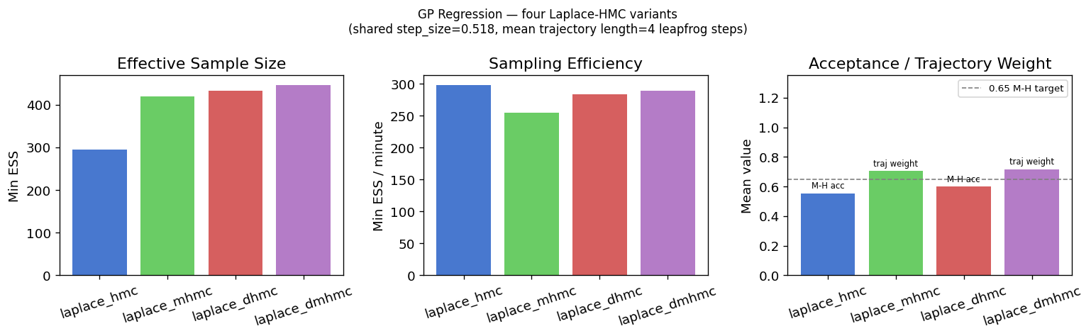

Reading the results. The acceptance rate panel reveals something important: laplace_hmc can show acceptable M-H acceptance rate yet produce a very low ESS. This could be the classic periodic-orbit pathology — a fixed trajectory length that happens to nearly return to the starting point, causing the chain to take tiny effective steps despite technically accepting. laplace_dhmc breaks the orbit by randomising the step count each transition, so even the same step size yields much better mixing. Multinomial variants (laplace_mhmc, laplace_dmhmc) also avoid the trap: by sampling a random point along the trajectory they implicitly vary the effective displacement, and is_accepted is always True so they never waste a trajectory.

This illustrates the core trade-off: if you can tune num_integration_steps carefully, laplace_hmc is the cheapest option; if you are unsure of the right trajectory length (common in practice), the dynamic and multinomial variants are more robust out of the box.

Quick-reference: when to use each variant.

Variant	Use when
`laplace_hmc`	Default when trajectory length is well-tuned; `window_adaptation` works directly
`laplace_mhmc`	Drop-in upgrade when M-H acceptance is low or ESS per gradient is poor
`laplace_dhmc`	Trajectory length is hard to tune; randomised steps break periodic-orbit traps
`laplace_dmhmc`	Combines both benefits — best robustness for unknown geometry