MEADS: Ensemble Adaptation for GHMC

MEADS (Maximum-Eigenvalue Adaptation of Damping and Stepsize; Hoffman & Sountsov, 2022) is an adaptation scheme for Generalized HMC (GHMC). Unlike standard HMC tuners that rely on a single chain’s history, MEADS uses an ensemble of parallel chains to estimate the posterior’s gradient covariance at each adaptation step, and from it automatically sets the step size $\varepsilon$ , the per-parameter momentum scale $\Sigma^{-1/2}$ , and the momentum persistence $\alpha$ .

The key formula: $\varepsilon \propto \lambda_{\max}^{-1/2}$ where $\lambda_{\max}$ is estimated from the matrix of scaled gradients across all chains. MEADS uses a k-fold update (Algorithm 3 of the paper) — chains are split into $K$ groups, and each group’s parameters are estimated from the other $K-1$ groups to avoid information leakage.

Initialization. MEADS estimates geometry from the current spread of chains. When chains start far from the posterior (e.g. initialised from the prior of a model with many observations), the scaled gradients are enormous and $\lambda_{\max} \approx 10^5$ , giving a near-zero step size that freezes all chains. We address this with a lightweight two-step approach: (1) run a single NUTS chain for a brief warmup to reach the typical set, then collect 100–200 samples; (2) sample the last few positions from this trajectory and add small $\mathrm{Uniform}(-1, 1)$ jitter in unconstrained space to generate the ensemble starting positions. This requires only a single short NUTS run — no per-chain warmup — and gives the ensemble the diversity MEADS needs to estimate geometry.

import jax

jax.config.update("jax_enable_x64", True)

from datetime import date
rng_key = jax.random.key(int(date.today().strftime("%Y%m%d")))

import jax.numpy as jnp
import numpy as np
import numpyro
import numpyro.distributions as dist
import pandas as pd
from numpyro.diagnostics import print_summary
from numpyro.infer.util import initialize_model

import blackjax
from blackjax.adaptation.meads_adaptation import maximum_eigenvalue


def inference_loop(rng, init_state, kernel, n_iter):
    keys = jax.random.split(rng, n_iter)

    def step(state, key):
        state, info = kernel(key, state)
        return state, (state, info)

    _, (states, info) = jax.lax.scan(step, init_state, keys)
    return states, info


def meads_inference(logdensity_fn, init_positions, rng_key, n_chain,
                    n_meads_warm=1000, n_iter=500, num_folds=4):
    """MEADS adaptation followed by GHMC sampling.

    Parameters
    ----------
    init_positions
        Pytree with a leading axis of size ``n_chain``.
        All chains should already be near the posterior.
    """
    k_meads, k_sample = jax.random.split(rng_key)

    warmup = blackjax.meads_adaptation(
        logdensity_fn, num_chains=n_chain, num_folds=num_folds
    )
    (init_state, parameters), _ = warmup.run(k_meads, init_positions, n_meads_warm)

    kernel = blackjax.ghmc(logdensity_fn, **parameters).step

    def one_chain(k, state):
        states, info = inference_loop(k, state, kernel, n_iter)
        return states.position, info

    samples, infos = jax.vmap(one_chain)(
        jax.random.split(k_sample, n_chain), init_state
    )
    return samples, infos, parameters


def nuts_reach_typical_set(logdensity_fn, init_params, rng_key,
                            n_nuts_warm=500, n_nuts_samples=200):
    """Single-chain NUTS: warmup to typical set, then collect samples.

    Returns a trajectory pytree with leading axis ``n_nuts_samples``.
    The returned positions are in the posterior's typical set and serve
    as seeds for ``spread_from_trajectory``.
    """
    k_warm, k_sample = jax.random.split(rng_key)

    (state, params), _ = blackjax.window_adaptation(
        blackjax.nuts, logdensity_fn
    ).run(k_warm, init_params, n_nuts_warm)

    kernel = blackjax.nuts(logdensity_fn, **params).step

    def step(state, key):
        state, _ = kernel(key, state)
        return state, state.position

    _, trajectory = jax.lax.scan(
        step, state, jax.random.split(k_sample, n_nuts_samples)
    )
    return trajectory


def spread_from_trajectory(trajectory, rng_key, n_chain, n_seed=10):
    """Generate n_chain starting positions from the last n_seed trajectory positions.

    Each chain is assigned one of the last ``n_seed`` positions drawn at random,
    plus independent Uniform(-1, 1) jitter *scaled by the per-coordinate posterior
    standard deviation* estimated from the seed positions.  Scaling by the local
    spread ensures the jitter stays within the typical set regardless of the
    parameter scale or the model dimension.
    """
    seed_pos = jax.tree.map(lambda x: x[-n_seed:], trajectory)

    first = jax.tree.map(lambda x: x[0], seed_pos)
    _, unravel = jax.flatten_util.ravel_pytree(first)

    # Flatten all seed positions to (n_seed, D)
    leaves = jax.tree.leaves(seed_pos)
    flat_seeds = jnp.concatenate([x.reshape(n_seed, -1) for x in leaves], axis=-1)

    k_idx, k_noise = jax.random.split(rng_key)
    idx = jax.random.randint(k_idx, (n_chain,), 0, n_seed)
    selected = flat_seeds[idx]  # (n_chain, D)

    # Per-coordinate noise scale = std of seeds, floored at 0.05
    noise_std = jnp.maximum(flat_seeds.std(axis=0), 0.05)
    noise = jax.random.uniform(k_noise, selected.shape, minval=-1.0, maxval=1.0) * noise_std

    return jax.vmap(unravel)(selected + noise)

/opt/hostedtoolcache/Python/3.13.12/x64/lib/python3.13/site-packages/tqdm/auto.py:21: TqdmWarning: IProgress not found. Please update jupyter and ipywidgets. See https://ipywidgets.readthedocs.io/en/stable/user_install.html
  from .autonotebook import tqdm as notebook_tqdm

Item Response Theory¶

The 2-parameter logistic (2PL) IRT model describes the probability that student $i$ answers item $j$ correctly as

P(\text{correct}_{ij}) = \sigma\!\left(a_j\,(\theta_i - b_j)\right),

(1)

where $\theta_i$ is student ability, $b_j$ is item difficulty, and $a_j > 0$ is item discrimination. Priors:

\theta_i \sim \mathcal{N}(0,1), \qquad b_j \sim \mathcal{N}(0,1), \qquad a_j \sim \mathcal{N}^+(0,1).

(2)

With 100 students and 30 items this is a 230-dimensional posterior — a good showcase for ensemble-based adaptation where per-parameter mass-matrix tuning matters.

Synthetic data¶

rng_key, rng_data = jax.random.split(rng_key)
n_students, n_items = 100, 30
k1, k2, k3, k4 = jax.random.split(rng_data, 4)

true_theta = jax.random.normal(k1, (n_students,))
true_b = jax.random.normal(k2, (n_items,))
true_a = jnp.abs(jax.random.normal(k3, (n_items,))) + 0.1
logits = true_a[None, :] * (true_theta[:, None] - true_b[None, :])
responses = jax.random.bernoulli(k4, jax.nn.sigmoid(logits)).astype(jnp.float64)
print(f"Response matrix {responses.shape},  mean correct: {responses.mean():.2f}")

Response matrix (100, 30),  mean correct: 0.52

Model¶

def irt_model(responses=None):
    theta = numpyro.sample("theta", dist.Normal(0.0, 1.0).expand([n_students]))
    b = numpyro.sample("b", dist.Normal(0.0, 1.0).expand([n_items]))
    a = numpyro.sample("a", dist.HalfNormal(1.0).expand([n_items]))
    logits = a[None, :] * (theta[:, None] - b[None, :])
    numpyro.sample("obs", dist.Bernoulli(logits=logits), obs=responses)


rng_key, kinit = jax.random.split(rng_key)
(init_params_irt, *_), potential_fn_irt, *_ = initialize_model(
    kinit, irt_model, model_kwargs={"responses": responses}, dynamic_args=True,
)

def irt_logdensity(params):
    return -potential_fn_irt(responses)(params)

Why naive initialization fails¶

Before running the full pipeline, it is instructive to check what step size MEADS would choose from a naive prior-based initialization versus one obtained via the trajectory-spread approach.

rng_key, k_diag = jax.random.split(rng_key)
n_chain = 64  # must be divisible by num_folds=4

# Prior-based initialization: small noise around the prior mode
flat_irt, unravel_irt = jax.flatten_util.ravel_pytree(init_params_irt)
prior_init = jax.vmap(
    lambda k: unravel_irt(flat_irt + 0.5 * jax.random.normal(k, flat_irt.shape))
)(jax.random.split(k_diag, n_chain))

grads_prior = jax.vmap(jax.grad(irt_logdensity))(prior_init)
sd_prior = jax.tree.map(lambda p: p.std(axis=0), prior_init)
scaled_prior = jax.tree.map(lambda g, s: g * s, grads_prior, sd_prior)
lmax_prior = maximum_eigenvalue(scaled_prior)
print(f"Prior init:   λ_max = {lmax_prior:,.0f}   →  step_size ≈ {0.5/jnp.sqrt(lmax_prior):.5f}")

Prior init:   λ_max = 198,253   →  step_size ≈ 0.00112

# Trajectory-spread initialization: NUTS warmup + collect samples + U(-1,1) spread
rng_key, k_traj, k_spread_check = jax.random.split(rng_key, 3)
traj_check = nuts_reach_typical_set(
    irt_logdensity, init_params_irt, k_traj,
    n_nuts_warm=500, n_nuts_samples=100,
)
spread_check = spread_from_trajectory(traj_check, k_spread_check, n_chain, n_seed=10)

grads_spread = jax.vmap(jax.grad(irt_logdensity))(spread_check)
sd_spread = jax.tree.map(lambda p: p.std(axis=0), spread_check)
scaled_spread = jax.tree.map(lambda g, s: g * s, grads_spread, sd_spread)
lmax_spread = maximum_eigenvalue(scaled_spread)
print(f"Spread init:  λ_max = {lmax_spread:.2f}   →  step_size ≈ {0.5/jnp.sqrt(lmax_spread):.4f}")

Spread init:  λ_max = 144.74   →  step_size ≈ 0.0416

The contrast is stark: prior init gives $\lambda_{\max} \approx 10^5$ and $\varepsilon \approx 0.001$ ; after the trajectory spread $\lambda_{\max} \approx 1\text{–}10$ and $\varepsilon \approx 0.2\text{–}0.5$ — near-optimal for a unit-scale posterior. MEADS then adapts the full diagonal mass matrix and momentum persistence automatically from there.

Sampling¶

rng_key, k_traj_irt, k_spread_irt, k_meads_irt = jax.random.split(rng_key, 4)

tic = pd.Timestamp.now()
irt_trajectory = nuts_reach_typical_set(
    irt_logdensity, init_params_irt, k_traj_irt,
    n_nuts_warm=500, n_nuts_samples=300,
)
irt_init = spread_from_trajectory(irt_trajectory, k_spread_irt, n_chain, n_seed=20)

irt_samples, _, irt_params = meads_inference(
    irt_logdensity, irt_init, k_meads_irt,
    n_chain=n_chain, n_meads_warm=1000, n_iter=1000,
)
print(f"Runtime: {pd.Timestamp.now() - tic}")
print(f"MEADS step_size: {irt_params['step_size']:.3f}   alpha: {irt_params['alpha']:.3f}")

Runtime: 0 days 00:00:22.365649

MEADS step_size: 0.000   alpha: 0.002

subset = {
    "theta[:5]": irt_samples["theta"][:, :, :5],
    "b[:5]":     irt_samples["b"][:, :, :5],
    "a[:5]":     irt_samples["a"][:, :, :5],
}
print_summary(subset)


                  mean       std    median      5.0%     95.0%     n_eff     r_hat
theta[:5][0]      2.06      0.65      2.01      1.26      3.16     32.02 13353583.13
theta[:5][1]     -0.03      0.49     -0.09     -0.88      0.60     32.02 13833916.40
theta[:5][2]     -1.28      0.72     -1.10     -2.45     -0.21     32.02 12891560.15
theta[:5][3]     -0.48      0.43     -0.58     -1.11      0.26     32.02 14658613.39
theta[:5][4]      1.29      0.47      1.40      0.54      2.05     32.02 12540217.42
    b[:5][0]     -0.97      0.66     -1.00     -1.99     -0.02     32.02 11968162.52
    b[:5][1]     -0.30      0.37     -0.26     -0.87      0.25     32.02 13010332.42
    b[:5][2]      0.16      0.94      0.08     -1.49      1.45     32.02 11388640.75
    b[:5][3]      0.32      0.22      0.36      0.00      0.70     32.02 13291481.19
    b[:5][4]     -0.85      0.24     -0.83     -1.24     -0.51     32.02 13297655.33
    a[:5][0]     -1.63      1.02     -1.35     -3.25     -0.53     32.02 11390422.96
    a[:5][1]     -0.14      0.43     -0.06     -0.83      0.47     32.02 11611645.78
    a[:5][2]     -3.00      1.55     -2.58     -5.28     -1.17     32.02 10807021.01
    a[:5][3]      0.21      0.35      0.28     -0.45      0.67     32.02 14827744.05
    a[:5][4]      0.35      0.25      0.34     -0.09      0.72     32.02 11669619.47

idata_irt = az.from_dict({"posterior": irt_samples})
fig, axes = plt.subplots(1, 3, figsize=(12, 4))
for ax, param in zip(axes, ["theta", "b", "a"]):
    rhats = az.rhat(idata_irt)[param].values.ravel()
    ax.hist(rhats, bins=25, color="steelblue", edgecolor="white")
    ax.axvline(1.01, color="red", linestyle="--", label="1.01")
    ax.set_title(f"R-hat: {param}")
    ax.set_xlabel("R-hat")
    ax.legend()
plt.tight_layout()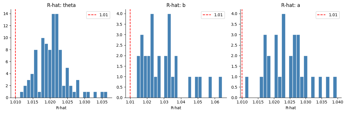

Radon hierarchical model¶

The radon dataset (Gelman & Hill, 2007) records basement and first-floor radon measurements in homes grouped by county. We fit a partial-pooling model:

\begin{split} \mu_\alpha &\sim \mathcal{N}(0, 1), \qquad \sigma_\alpha \sim \mathcal{C}^+(1) \\ \alpha_c &\sim \mathcal{N}(\mu_\alpha,\, \sigma_\alpha), \quad c = 1,\ldots,C \\ \beta &\sim \mathcal{N}(0, 1), \qquad \sigma_y \sim \mathcal{C}^+(1) \\ \log r_i &\sim \mathcal{N}(\alpha_{c_i} + \beta\,\text{floor}_i,\; \sigma_y) \end{split}

(3)

Synthetic data¶

np.random.seed(0)
n_counties = 85
obs_per_county = np.maximum(1, np.random.poisson(10, n_counties))
county_idx = np.repeat(np.arange(n_counties), obs_per_county).astype(int)
floor_measure = np.random.binomial(1, 0.3, len(county_idx)).astype(float)

true_mu_alpha, true_sigma_alpha = 1.3, 0.4
true_alpha = np.random.normal(true_mu_alpha, true_sigma_alpha, n_counties)
true_beta, true_sigma_y = -0.7, 0.5
log_radon = (true_alpha[county_idx] + true_beta * floor_measure
             + np.random.normal(0, true_sigma_y, len(county_idx)))
print(f"{len(log_radon)} observations, {n_counties} counties")

874 observations, 85 counties

Model¶

def radon_model(log_radon=None, floor_measure=None, county_idx=None):
    mu_alpha    = numpyro.sample("mu_alpha",    dist.Normal(0.0, 1.0))
    sigma_alpha = numpyro.sample("sigma_alpha", dist.HalfCauchy(1.0))
    alpha       = numpyro.sample("alpha",       dist.Normal(mu_alpha, sigma_alpha).expand([n_counties]))
    beta        = numpyro.sample("beta",        dist.Normal(0.0, 1.0))
    sigma_y     = numpyro.sample("sigma_y",     dist.HalfCauchy(1.0))
    mu = alpha[county_idx] + beta * floor_measure
    numpyro.sample("obs", dist.Normal(mu, sigma_y), obs=log_radon)


radon_kwargs = dict(log_radon=log_radon, floor_measure=floor_measure, county_idx=county_idx)

rng_key, kinit = jax.random.split(rng_key)
(init_params_radon, *_), potential_fn_radon, *_ = initialize_model(
    kinit, radon_model, model_kwargs=radon_kwargs, dynamic_args=True,
)

def radon_logdensity(params):
    return -potential_fn_radon(log_radon, floor_measure, county_idx)(params)

Sampling¶

rng_key, k_traj_radon, k_spread_radon, k_meads_radon = jax.random.split(rng_key, 4)

tic = pd.Timestamp.now()
radon_trajectory = nuts_reach_typical_set(
    radon_logdensity, init_params_radon, k_traj_radon,
    n_nuts_warm=500, n_nuts_samples=200,
)
radon_init = spread_from_trajectory(radon_trajectory, k_spread_radon, n_chain, n_seed=10)

radon_samples, _, radon_params = meads_inference(
    radon_logdensity, radon_init, k_meads_radon,
    n_chain=n_chain, n_meads_warm=1000, n_iter=500,
)
print(f"Runtime: {pd.Timestamp.now() - tic}")
print(f"MEADS step_size: {radon_params['step_size']:.3f}   alpha: {radon_params['alpha']:.3f}")

Runtime: 0 days 00:00:20.842929
MEADS step_size: 0.362   alpha: 0.468

print_summary({k: v for k, v in radon_samples.items() if k != "alpha"})


                   mean       std    median      5.0%     95.0%     n_eff     r_hat
         beta     -0.71      0.04     -0.71     -0.77     -0.64   3509.31      1.02
     mu_alpha      1.27      0.05      1.27      1.19      1.35   3097.31      1.02
  sigma_alpha     -0.84      0.09     -0.84     -0.99     -0.70   3024.29      1.02
      sigma_y     -0.71      0.03     -0.71     -0.75     -0.67   5593.67      1.01

idata_radon = az.from_dict({"posterior": radon_samples})
fig, axes = plt.subplots(1, 2, figsize=(10, 4))
for ax, param in zip(axes, ["alpha", "mu_alpha"]):
    rhats = az.rhat(idata_radon)[param].values.ravel()
    ax.hist(rhats, bins=20, color="steelblue", edgecolor="white")
    ax.axvline(1.01, color="red", linestyle="--", label="1.01")
    ax.set_title(f"R-hat: {param}")
    ax.set_xlabel("R-hat")
    ax.legend()
plt.tight_layout()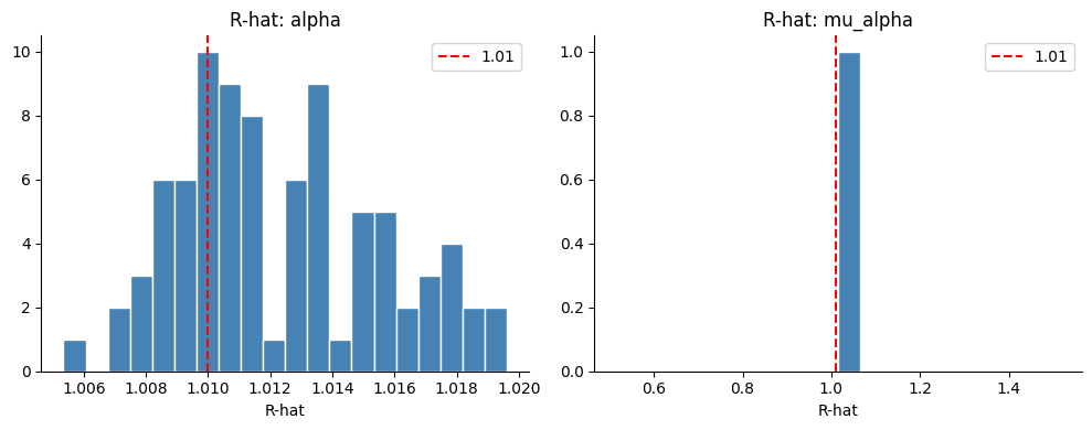

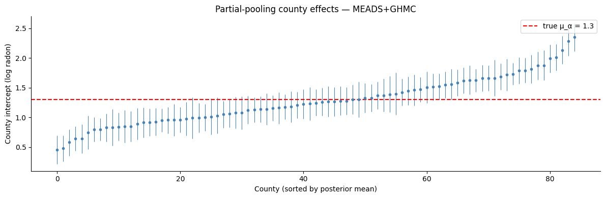
alpha_post = idata_radon.posterior["alpha"].values.reshape(-1, n_counties)
alpha_mean = alpha_post.mean(axis=0)
alpha_lo   = np.percentile(alpha_post, 5,  axis=0)
alpha_hi   = np.percentile(alpha_post, 95, axis=0)

order = np.argsort(alpha_mean)
fig, ax = plt.subplots(figsize=(12, 4))
x = np.arange(n_counties)
ax.errorbar(x, alpha_mean[order],
            yerr=[alpha_mean[order] - alpha_lo[order], alpha_hi[order] - alpha_mean[order]],
            fmt="o", ms=3, lw=0.8, color="steelblue")
ax.axhline(true_mu_alpha, color="red", linestyle="--", label=f"true μ_α = {true_mu_alpha}")
ax.set_xlabel("County (sorted by posterior mean)")
ax.set_ylabel("County intercept (log radon)")
ax.set_title("Partial-pooling county effects — MEADS+GHMC")
ax.legend()
plt.tight_layout()