Microcanonical Langevin Monte Carlo

This is an algorithm based on MCHMC and MCLMC papers. A website with detailed information can be found here.

The idea is that we have a distribution $p(x)$ from which we want to sample. We numerically integrate the following SDE; the samples we obtain converge (in the limit of many steps and small step size) to samples from the target distribution.

\frac{d}{dt}\begin{bmatrix} x \\ u \end{bmatrix} = \begin{bmatrix} u \\ -P(u)(\nabla S(x)/(d − 1)) + \eta P(u)dW \end{bmatrix}

(1)

Here $x \in \mathbb{R}^n$ is the variable of interest (i.e. the variable of the target distribution $p$ ), $u \in \mathbb{S}^{n-1}$ is the momentum (i.e. $u$ lives in $\mathbb{R}^n$ but is constrained to have fixed norm), $S(x)$ is the negative log PDF of the distribution from which we are sampling, and $P(u)=(I-uu^T)$ is the projection operator. The term $\eta P(u)dW$ describes spherically symmetric noise on the $n-1$ sphere $\mathbb{S}^{n-1}$ . After $u$ is marginalized out, this converges to the target PDF, $p(x) \propto e^{-S(x)}$ .

How to run MCLMC in BlackJax¶

MCLMC has two parameters:

Typical momentum decoherence scale $L$ . This adds some noise to the direction of the velocity after every step. $L = \infty$ means no noise, $L = 0$ is full refreshement after every step.
Stepsize $\epsilon$ of the discretization of the dynamics. While the continuous dynamics converge exactly on the target distribution, the discrete dynamics inject bias into the resulting distribution. As such, we want to find the ideal tradeoff: $\epsilon$ small enough for bias to be minimal, but large enough for computational efficiency.

MCLMC in Blackjax comes with a tuning algorithm which attempts to find optimal values for both of these parameters. This must be used for good performance.

An example is given below, of tuning and running a chain for a 1000 dimensional Gaussian target (of which a 2 dimensional marginal is plotted):

import matplotlib.pyplot as plt

plt.rcParams["axes.spines.right"] = False
plt.rcParams["axes.spines.top"] = False
plt.rcParams["font.size"] = 19

import jax
import blackjax
import numpy as np
import jax.numpy as jnp
from datetime import date
import numpyro
import numpyro.distributions as dist

from numpyro.infer.util import initialize_model

rng_key = jax.random.key(int(date.today().strftime("%Y%m%d")))

/opt/hostedtoolcache/Python/3.13.12/x64/lib/python3.13/site-packages/tqdm/auto.py:21: TqdmWarning: IProgress not found. Please update jupyter and ipywidgets. See https://ipywidgets.readthedocs.io/en/stable/user_install.html
  from .autonotebook import tqdm as notebook_tqdm

def run_mclmc(logdensity_fn, num_steps, initial_position, key, transform, desired_energy_variance= 5e-4):
    init_key, tune_key, run_key = jax.random.split(key, 3)

    # create an initial state for the sampler
    initial_state = blackjax.mcmc.mclmc.init(
        position=initial_position, logdensity_fn=logdensity_fn, rng_key=init_key
    )

    # build the kernel
    kernel = lambda inverse_mass_matrix : blackjax.mcmc.mclmc.build_kernel(
        logdensity_fn=logdensity_fn,
        integrator=blackjax.mcmc.integrators.isokinetic_mclachlan,
        inverse_mass_matrix=inverse_mass_matrix,
    )

    # find values for L and step_size
    (
        blackjax_state_after_tuning,
        blackjax_mclmc_sampler_params,
        _
    ) = blackjax.mclmc_find_L_and_step_size(
        mclmc_kernel=kernel,
        num_steps=num_steps,
        state=initial_state,
        rng_key=tune_key,
        diagonal_preconditioning=False,
        desired_energy_var=desired_energy_variance
    )

    # use the quick wrapper to build a new kernel with the tuned parameters
    sampling_alg = blackjax.mclmc(
        logdensity_fn,
        L=blackjax_mclmc_sampler_params.L,
        step_size=blackjax_mclmc_sampler_params.step_size,
    )

    # run the sampler
    _, samples = blackjax.util.run_inference_algorithm(
        rng_key=run_key,
        initial_state=blackjax_state_after_tuning,
        inference_algorithm=sampling_alg,
        num_steps=num_steps,
        transform=transform,
        progress_bar=True,
    )

    return samples, blackjax_state_after_tuning, blackjax_mclmc_sampler_params, run_key

# run the algorithm on a high dimensional gaussian, and show two of the dimensions

logdensity_fn = lambda x: -0.5 * jnp.sum(jnp.square(x))
num_steps = 10000
transform = lambda state, info: state.position[:2]


sample_key, rng_key = jax.random.split(rng_key)
samples, initial_state, params, chain_key = run_mclmc(
    logdensity_fn=logdensity_fn,
    num_steps=num_steps,
    initial_position=jnp.ones((1000,)),
    key=sample_key,
    transform=transform,
)
samples.mean()

Array(-0.00957088, dtype=float32)

plt.scatter(x=samples[:, 0], y=samples[:, 1], alpha=0.1)
plt.axis("equal")
plt.title("Scatter Plot of Samples")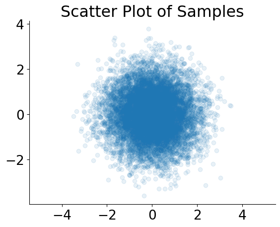

def visualize_results_gauss(samples, label, color):
  x1 = samples[:, 0]
  plt.hist(x1, bins= 30, density= True, histtype= 'step', lw= 4, color= color, label= label)


def ground_truth_gauss():
  # ground truth
  t= np.linspace(-4, 4, 200)
  plt.plot(t, np.exp(-0.5 * np.square(t)) / np.sqrt(2 *  np.pi), color= 'black', label= 'exact')
  plt.xlabel(r'$x_1$')
  plt.ylabel(r'$p(x_1$)')
  plt.legend()
  plt.show()

visualize_results_gauss(samples, 'MCLMC', 'teal')
ground_truth_gauss()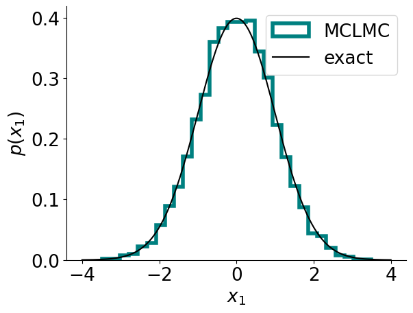

Note that the number of samples is relatively large compared to the number of samples typically used by say NUTS. This is because for MCLMC each sample corresponds to one integration step, while for NUTS each sample corresponds to multiple integration steps (typically to up to 1024). What determines the runtime is the number of integration steps, not the number of samples.

How to analyze the results of your MCLMC run¶

Validate the choice of $\epsilon$ ¶

A natural sanity check is to see if reducing $\epsilon$ changes the inferred distribution to an extent you care about. For example, we can inspect the 1D marginal with a stepsize $\epsilon$ as above, and compare it to a stepsize $\epsilon/2$ (and double the number of steps). We show this comparison below:

new_params = params._replace(step_size= params.step_size / 2)
new_num_steps = num_steps * 2

sampling_alg = blackjax.mclmc(
    logdensity_fn,
    L=new_params.L,
    step_size=new_params.step_size,
)

# run the sampler
_, new_samples = blackjax.util.run_inference_algorithm(
    rng_key= chain_key,
    initial_state=initial_state,
    inference_algorithm=sampling_alg,
    num_steps=new_num_steps,
    transform=transform,
    progress_bar=True,
)

visualize_results_gauss(new_samples, 'MCLMC', 'red')
visualize_results_gauss(samples, 'MCLMC', 'teal')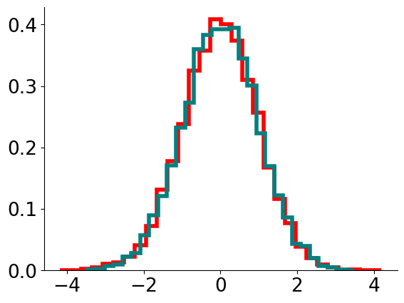

So here the change has little effect in this case.

A more complex example¶

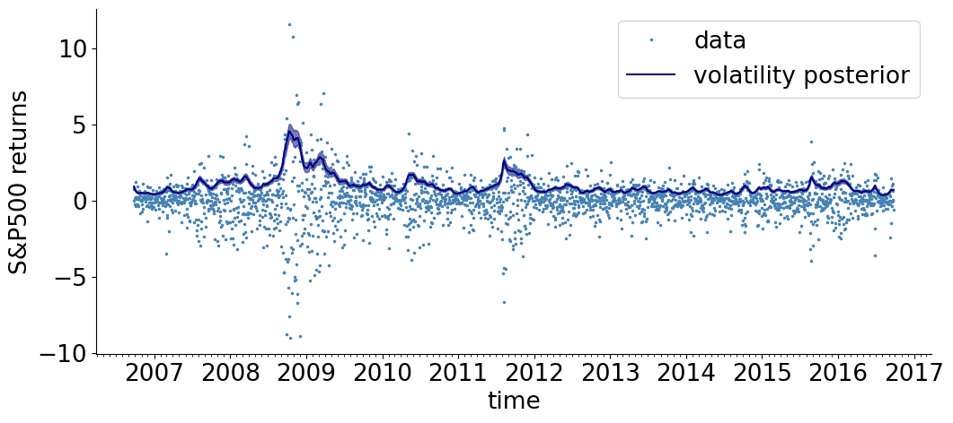
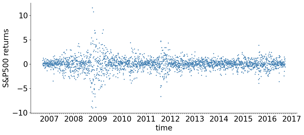
We now consider a more complex model, of stock volatility.

The returns $r_n$ are modeled by a Student’s-t distribution whose scale (volatility) $R_n$ is time varying and unknown. The prior for $\log R_n$ is a Gaussian random walk, with an exponential distribution of the random walk step-size $\sigma$ . An exponential prior is also taken for the Student’s-t degrees of freedom $\nu$ . The generative process of the data is:

\begin{align} &r_n / R_n \sim \text{Student's-t}(\nu) \qquad &&\nu \sim \text{Exp}(\lambda = 1/10) \\ \nonumber &\log R_n \sim \mathcal{N}(\log R_{n-1}, \sigma) \qquad &&\sigma \sim \text{Exp}(\lambda = 1/0.02). \end{align}

(2)

Our task is to find the posterior of the parameters $\{R_n\}_{n =1}^N$ , $\sigma$ and $\nu$ , given the observed data $\{r_n\}_{n =1}^N$ .

First, we get the data, define a model using NumPyro, and draw samples:

import matplotlib.dates as mdates
from numpyro.examples.datasets import SP500, load_dataset
from numpyro.distributions import StudentT

# get the data
_, fetch = load_dataset(SP500, shuffle=False)
SP500_dates, SP500_returns = fetch()
dates = mdates.num2date(mdates.datestr2num(SP500_dates))



def setup():
  # figure setup,
  plt.figure(figsize = (12, 5))
  ax = plt.subplot()
  ax.spines['right'].set_visible(False) #remove the upper and the right axis lines
  ax.spines['top'].set_visible(False)

  ax.xaxis.set_major_locator(mdates.YearLocator()) #dates on the xaxis
  ax.xaxis.set_major_formatter(mdates.DateFormatter("%Y"))
  ax.xaxis.set_minor_locator(mdates.MonthLocator())

  # plot data
  plt.plot(dates, SP500_returns, '.', markersize = 3, color= 'steelblue', label= 'data')
  plt.xlabel('time')
  plt.ylabel('S&P500 returns')


setup()

Downloading - https://github.com/pyro-ppl/datasets/blob/master/SP500.csv?raw=true.

Download complete.

def from_numpyro(model, rng_key, model_args):
  init_params, potential_fn_gen, *_ = initialize_model(
      rng_key,
      model,
      model_args= model_args,
      dynamic_args=True,
  )

  logdensity_fn = lambda position: -potential_fn_gen(*model_args)(position)
  initial_position = init_params.z

  return logdensity_fn, initial_position


def stochastic_volatility(sigma_mean, nu_mean):
    """numpyro model"""
    sigma = numpyro.sample("sigma", dist.Exponential(1./sigma_mean))
    nu = numpyro.sample("nu", dist.Exponential(1./nu_mean))
    s = numpyro.sample("s", dist.GaussianRandomWalk(scale=sigma, num_steps=jnp.shape(SP500_returns)[0])) # = log R
    numpyro.sample("r", dist.StudentT(df=nu, loc=0.0, scale=jnp.exp(s)), obs= SP500_returns)


model_args = (0.02, 10.)
rng_key = jax.random.key(42)

logp_sv, x_init = from_numpyro(stochastic_volatility, rng_key, model_args)

num_steps = 20000

samples, initial_state, params, chain_key = run_mclmc(logdensity_fn= logp_sv, num_steps= num_steps, initial_position= x_init, key= sample_key, transform=lambda state, info: state.position)

def visualize_results_sv(samples, color, label):

  R = np.exp(np.array(samples['s'])) # take an exponent to get R
  lower_quantile, median, upper_quantile = np.quantile(R, [0.25, 0.5, 0.75], axis= 0)

  # plot posterior
  plt.plot(dates, median, color= color, label = label)
  plt.fill_between(dates, lower_quantile, upper_quantile, color= color, alpha=0.5)


setup()

visualize_results_sv(samples, color= 'navy', label= 'volatility posterior')

plt.legend()
plt.show()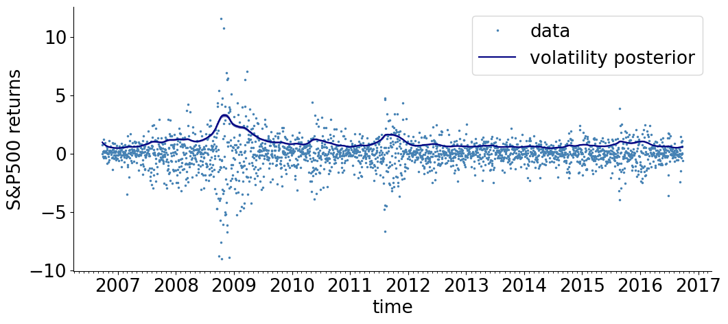

new_params = params._replace(step_size = params.step_size/2)
new_num_steps = num_steps * 2

sampling_alg = blackjax.mclmc(
    logp_sv,
    L=new_params.L,
    step_size=new_params.step_size,
)



# # run the sampler
_, new_samples = blackjax.util.run_inference_algorithm(
    rng_key=chain_key,
    initial_state=initial_state,
    inference_algorithm=sampling_alg,
    num_steps=new_num_steps,
    transform=lambda state, info : state.position,
    progress_bar=True,
)

setup()
visualize_results_sv(new_samples,'red', 'MCLMC', )
visualize_results_sv(samples,'teal', 'MCLMC (stepsize/2)', )

plt.legend()
plt.show()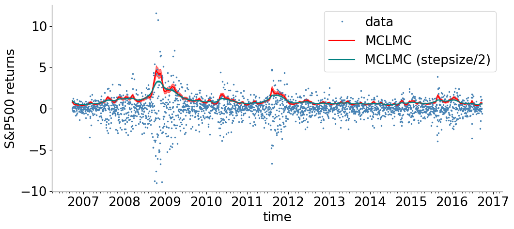

Here, we have again inspected the effect of halving $\epsilon$ . This looks OK, but suppose we are interested in the hierarchial parameters in particular, which tend to be harder to infer. We now inspect the marginal of a hierarchical parameter:

def visualize_results_sv_marginal(samples, color, label):
    # plt.subplot(1, 2, 1)
    # plt.hist(samples['nu'], bins = 20, histtype= 'step', lw= 4, density= True, color= color, label= label)
    # plt.xlabel(r'$\nu$')
    # plt.ylabel(r'$p(\nu \vert \mathrm{data})$')

    plt.subplot(1, 2, 2)
    plt.hist(samples['sigma'], bins = 20, histtype= 'step', lw= 4, density= True, color= color, label= label)
    plt.xlabel(r'$\sigma$')
    plt.ylabel(r'$p(\sigma \vert \mathrm{data})$')


plt.figure(figsize = (10, 4))
visualize_results_sv_marginal(samples, color= 'teal', label= 'MCLMC')
visualize_results_sv_marginal(new_samples, color= 'red', label= 'MCLMC (stepsize/2)')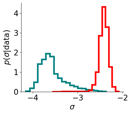

If we care about this parameter in particular, we should reduce step size further, until the difference disappears.

Adjusted MCLMC¶

Blackjax also provides an adjusted version of the algorithm, based on this paper. This also has two hyperparameters, step_size and L. L is related to the L parameter of the unadjusted version, but not identical (It determines the length of a proposal, and since momentum is resampled after a proposal, length of proposal determines the momentum decoherence rate). It is also possible to have Langevin noise during the trajectory, although we don’t see improvements here.

The tuning algorithm is also similar, but uses a dual averaging scheme to tune the step size. We find in practice that a target MH acceptance rate of 0.9 is a good choice.

Our recommendation is to use the unadjusted version when possible, but if you really believe you need the algorithm to be asymptotically unbiased (it’s not obvious why you would), you should use the adjusted version, with mass matrix preconditioning, randomized trajectory length and no in-proposal Langevin noise. We encapsulate these best practices in run_adjusted_mcmc below:

from blackjax.mcmc.adjusted_mclmc_dynamic import rescale
from blackjax.util import run_inference_algorithm

def run_adjusted_mclmc_dynamic(
    logdensity_fn,
    num_steps,
    initial_position,
    key,
    transform=lambda state, _ : state.position,
    diagonal_preconditioning=True,
    random_trajectory_length=True,
    L_proposal_factor=jnp.inf
):

    init_key, tune_key, run_key = jax.random.split(key, 3)

    initial_state = blackjax.mcmc.adjusted_mclmc_dynamic.init(
        position=initial_position,
        logdensity_fn=logdensity_fn,
        random_generator_arg=init_key,
    )

    if random_trajectory_length:
        integration_steps_fn = lambda avg_num_integration_steps: lambda k: jnp.ceil(
            jax.random.uniform(k) * rescale(avg_num_integration_steps))
    else:
        integration_steps_fn = lambda avg_num_integration_steps: lambda _: jnp.ceil(avg_num_integration_steps)

    kernel = lambda rng_key, state, avg_num_integration_steps, step_size, inverse_mass_matrix: blackjax.mcmc.adjusted_mclmc_dynamic.build_kernel(
        integration_steps_fn=integration_steps_fn(avg_num_integration_steps),
        inverse_mass_matrix=inverse_mass_matrix,
    )(
        rng_key=rng_key,
        state=state,
        step_size=step_size,
        logdensity_fn=logdensity_fn,
        L_proposal_factor=L_proposal_factor,
    )

    target_acc_rate = 0.9 # our recommendation

    (
        blackjax_state_after_tuning,
        blackjax_mclmc_sampler_params,
        _
    ) = blackjax.adjusted_mclmc_find_L_and_step_size(
        mclmc_kernel=kernel,
        num_steps=num_steps,
        state=initial_state,
        rng_key=tune_key,
        target=target_acc_rate,
        frac_tune1=0.1,
        frac_tune2=0.1,
        frac_tune3=0.1, # our recommendation
        diagonal_preconditioning=diagonal_preconditioning,
    )

    step_size = blackjax_mclmc_sampler_params.step_size
    L = blackjax_mclmc_sampler_params.L

    alg = blackjax.adjusted_mclmc_dynamic(
        logdensity_fn=logdensity_fn,
        step_size=step_size,
        integration_steps_fn=lambda key: jnp.ceil(
            jax.random.uniform(key) * rescale(L / step_size)
        ),
        inverse_mass_matrix=blackjax_mclmc_sampler_params.inverse_mass_matrix,
        L_proposal_factor=L_proposal_factor,
    )

    _, out = run_inference_algorithm(
        rng_key=run_key,
        initial_state=blackjax_state_after_tuning,
        inference_algorithm=alg,
        num_steps=num_steps,
        transform=transform,
        progress_bar=False,
    )

    return out

# run the algorithm on a high dimensional gaussian, and show two of the dimensions

sample_key, rng_key = jax.random.split(rng_key)
samples = run_adjusted_mclmc_dynamic(
    logdensity_fn=lambda x: -0.5 * jnp.sum(jnp.square(x)),
    num_steps=1000,
    initial_position=jnp.ones((1000,)),
    key=sample_key,
)
plt.scatter(x=samples[:, 0], y=samples[:, 1], alpha=0.1)
plt.axis("equal")
plt.title("Scatter Plot of Samples")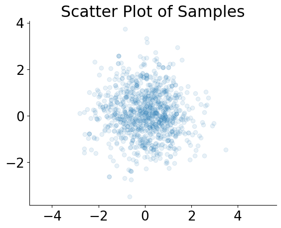

num_steps = 10000

adjusted_samples = run_adjusted_mclmc_dynamic(logdensity_fn= logp_sv, num_steps= num_steps, initial_position= x_init, key= sample_key)

setup()
visualize_results_sv(adjusted_samples, color= 'navy', label= 'volatility posterior')

plt.legend()
plt.show()