Comparing SMC and Persistent Sampling

This notebook extends the Use Tempered SMC to Improve Exploration of MCMC Methods and Tuning inner kernel parameters of SMC, exploring the theory and implementation of Persistent Sampling (PS) as described in Karamanis et al. (2025), and comparing it with standard tempered Sequential Monte Carlo (SMC) methods. We will compare four different methods:

SMC with a fixed tempering schedule
PS with a fixed tempering schedule
SMC with an adaptive tempering schedule
PS with an adaptive tempering schedule

Introduction¶

Sequential Monte Carlo (SMC)¶

SMC samplers propagate N particles through a sequence of probability distributions $p_t(\theta)$ for $t = 1, \ldots, T$ , using three main steps:

Reweighting: Adjust particle weights using importance sampling
Resampling: Discard low-weight particles and replicate high-weight ones
Moving: Apply MCMC steps to diversify particles

For Bayesian inference with temperature annealing:

p_t(\theta) = \frac{\mathcal{L}(\theta)^{\beta_t} \pi(\theta)}{Z_t}

(1)

where $0 = \beta_1 < \cdots < \beta_T = 1$ interpolates between prior $\pi(\theta)$ and posterior.

Persistent Sampling (PS)¶

PS extends SMC by retaining and reusing particles from all prior iterations, constructing a growing weighted ensemble. Key differences:

Mixture Distribution: At iteration $t$ , particles from previous iterations are treated as samples from:

\tilde{p}_t(\theta) = \frac{1}{t-1} \sum_{s=1}^{t-1} p_s(\theta)

(2)

Persistent Weights: Using multiple importance sampling, weights for particle $\theta^i_{t'}$ at iteration $t$ are:

W^i_{tt'} = \frac{\mathcal{L}(\theta^i_{t'})^{\beta_t}}{\frac{1}{t-1}\sum_{s=1}^{t-1} \mathcal{L}(\theta^i_{t'})^{\beta_s}/\hat{Z}_s} \cdot \frac{1}{\hat{Z}_t}

(3)

Resampling: N particles are resampled from $(t-1) \times N$ persistent particles

Key Advantages:

Reduced particle correlation after resampling
Lower variance estimates for marginal likelihood $Z$
Lower variance when calculating expectations
$\hat{f} = \sum_{t^\prime}^T \sum_{i}^N W^i_{T{t^\prime}} f(\theta^i_{t^\prime})$
(4)

Trade-offs:

Introduces small bias (proven to be consistent)
Higher memory footprint (stores all particles)
More arithmetic operations per iteration

Imports and Settings¶

import jax
import jax.numpy as jnp
import matplotlib.pyplot as plt
from jax.scipy.stats import multivariate_normal

import blackjax
import blackjax.smc.resampling as resampling
from blackjax.smc import extend_params

# Set random seed for reproducibility
key = jax.random.key(20251023)


# Plot settings
plt.rcParams["figure.figsize"] = (12, 8)
plt.rcParams["font.size"] = 10

Experimental Setup¶

We will use the same setup as in Use Tempered SMC to Improve Exploration of MCMC Methods. We have seen that SMC can efficiently sample from a multimodal distribution.

# Define target distribution
def V(x):
    """Potential for two-mode distribution."""
    return 5 * jnp.square(jnp.sum(x**2, axis=-1) - 1)


def log_likelihood_fn(x):
    """Log likelihood function."""
    return -V(x)


def log_prior_fn(x):
    """Log prior function."""
    d = x.shape[-1]
    return multivariate_normal.logpdf(x, jnp.zeros((d,)), jnp.eye(d))


def log_posterior_fn(x):
    """Log posterior function, the target distribution."""
    return log_likelihood_fn(x) + log_prior_fn(x)

# HMC parameters
hmc_parameters = dict(
    step_size=1e-4,
    inverse_mass_matrix=jnp.eye(1),
    num_integration_steps=50,
)


# Initialize particles for the samplers
num_particles = 10_000
initial_particles = jax.random.normal(key, (num_particles, 1))

SMC with Fixed Schedule¶

Now we’ll run standard SMC with a fixed tempering schedule. The tempering schedule and inference loop can be reused for PS.

# Tempering schedule
tempering_schedule = jnp.linspace(0.0, 1.0, 30)


# Inference loop for a fixed schedule
def fixed_schedule_loop(rng_key, sampler, initial_state, tempering_schedule):
    """Run SMC/PS with a fixed tempering schedule."""

    @jax.jit
    def one_step(carry, lmbda):
        state, key = carry
        key, subkey = jax.random.split(key, 2)
        state, _ = sampler.step(subkey, state, lmbda)
        # Return weights history for marginal likelihood computation
        return (state, key), None

    (final_state, _), weights_history = jax.lax.scan(
        one_step,
        (initial_state, rng_key),
        tempering_schedule,
    )

    return final_state, weights_history

%%time

# Initialize SMC sampler
smc_sampler = blackjax.tempered_smc(
    log_prior_fn,
    log_likelihood_fn,
    blackjax.hmc.build_kernel(),
    blackjax.hmc.init,
    extend_params(hmc_parameters),
    resampling.systematic,
    num_mcmc_steps=10,
)

# Run SMC with fixed schedule
key, smc_key = jax.random.split(key)
smc_initial_state = smc_sampler.init(initial_particles)
smc_final_state, _ = fixed_schedule_loop(
    smc_key,
    smc_sampler,
    smc_initial_state,
    tempering_schedule,
)

smc_final_weights = (
    smc_final_state.weights / jnp.sum(smc_final_state.weights)
).block_until_ready()
print(f"Final ESS (SMC): {1.0 / jnp.sum(smc_final_weights**2):.2f}\n")

Final ESS (SMC): 9991.15

CPU times: user 2min 47s, sys: 351 ms, total: 2min 47s
Wall time: 1min 51s

Persistent Sampling with Fixed Schedule¶

Now we run the same loop for the persistent sampling. Note that there are a few conditions and caveats for Persistent Sampling to function correctly:

For the reweighting scheme to work correctly, the prior density must be normalised to 1.
Related to the statement above, the tempering schedule must start at 0. Together with the normalised prior, this guarantees that $Z_0 = 1$ . Internally, this is enforced by adding a 0.0 to the beginning of the tempering schedule.
To keep track of the persistent particles in a JIT-compatible way, all arrays in the PSState must be padded to the length of the tempering schedule (+1 to account for the added 0.0 mentioned above). The values get filled in with each iteration of the sampler. For this reason, the persistent_sampling_smc requires an n_schedule which MUST match the length of the tempering schedule. This can lead to highly increased memory usage for long tempering schedules.
The padding is done internally when calling the init function. The padding value is 0.
The weights returned by ps_final_state.persistent weights are normalised to sum to ( $i \cdot N$ ). This is the appropriate normalization to calculate expectations values as defined in the introduction. However, to calculate the effective sample size using the common $\sum \frac{1}{W^2}$ equation, they first need to be normalized to 1.

Finally, the effective sample size of the final persistent ensemble can (and ideally will) be much larger than the number of particles per iteration.

%%time

# Initialize Persistent Sampling
ps_sampler = blackjax.persistent_sampling_smc(
    log_prior_fn,
    log_likelihood_fn,
    tempering_schedule.shape[0],
    blackjax.hmc.build_kernel(),
    blackjax.hmc.init,
    extend_params(hmc_parameters),
    resampling.systematic,
    num_mcmc_steps=10,
)

# Run Persistent Sampling with fixed schedule
key, ps_key = jax.random.split(key)
ps_initial_state = ps_sampler.init(initial_particles)
ps_final_state, _ = fixed_schedule_loop(
    ps_key,
    ps_sampler,
    ps_initial_state,
    tempering_schedule,
)

ps_final_weights = (
    ps_final_state.persistent_weights / jnp.sum(ps_final_state.persistent_weights)
).block_until_ready()
print(f"Final ESS (Persistent Sampling): {1.0 / jnp.sum(ps_final_weights**2):.2f} \n")

Final ESS (Persistent Sampling): 236925.39 

CPU times: user 1min 3s, sys: 261 ms, total: 1min 3s
Wall time: 28.6 s

Adaptive SMC¶

Now we run the adaptive algorithms where the tempering schedule is chosen automatically. For the adaptive algorithm inference loop, we use a while loop that terminates when a tempering paramter of 1 is reached, or a predefined number of iterations is exceeded.

def adaptive_schedule_loop(rng_key, sampler, cond, initial_state, max_iterations):
    """Run adaptive SMC until condition is met."""

    @jax.jit
    def one_step(carry):
        i, state, key = carry
        key, subkey = jax.random.split(key)
        state, _ = sampler.step(subkey, state)
        return i + 1, state, key

    n_iter, final_state, _ = jax.lax.while_loop(
        cond,
        one_step,
        (0, initial_state, rng_key),
    )

    if n_iter >= max_iterations:
        print(
            "Warning: Maximum number of iterations reached before lambda=1.0, "
            "the final state may not represent the target distribution. "
            "Check the final tempering parameter value."
        )

    return n_iter, final_state

%%time

max_iterations = 100
target_ess = 0.95

# Initialize Adaptive SMC sampler
adaptive_smc_sampler = blackjax.adaptive_tempered_smc(
    log_prior_fn,
    log_likelihood_fn,
    blackjax.hmc.build_kernel(),
    blackjax.hmc.init,
    extend_params(hmc_parameters),
    resampling.systematic,
    target_ess=target_ess,
    num_mcmc_steps=10,
)

# Define condition function for Adaptive SMC
def smc_cond(carry):
    """Returns True while lambda < 1.0 and iteration < max_iterations."""
    i, state, _ = carry
    return (state.tempering_param < 1.0) & (i < max_iterations)

# Run Adaptive SMC
key, adaptive_smc_key = jax.random.split(key)
adaptive_smc_initial_state = adaptive_smc_sampler.init(initial_particles)
adaptive_smc_n_iter, adaptive_smc_final_state = adaptive_schedule_loop(
    adaptive_smc_key,
    adaptive_smc_sampler,
    smc_cond,
    adaptive_smc_initial_state,
    max_iterations,
)


adaptive_smc_final_weights = (
    adaptive_smc_final_state.weights / jnp.sum(adaptive_smc_final_state.weights)
).block_until_ready()
print("Number of iterations (Adaptive SMC):", adaptive_smc_n_iter)
print(
    f"Final ESS (Adaptive SMC): {1.0 / jnp.sum(adaptive_smc_final_weights**2):.2f} \n"
)

Number of iterations (Adaptive SMC): 19
Final ESS (Adaptive SMC): 9985.92 

CPU times: user 53.1 s, sys: 187 ms, total: 53.3 s
Wall time: 29.3 s

Adaptive Persistent Sampling¶

The adaptive Persistent Sampling algorithm works similar to the adaptive SMC algorithm. However, there are a few noteworthy percularities:

Since the arrays for storing the persistent ensemble need to be preallocated, the max_iterations parameter is a requirement. The arrays get padded to the shape (max_iternations + 1, n_particles). Therefore a large value for max_iterations can lead to high memory usage. Note that there is no internal check for the sampler if the max iterations are exceeded, the values will simply be written to the last available spot in the preallocated array. One should therefore include a check in the inference loop condition.
The target ESS for Persistent Sampling can exceed 1, since we work with a larger ensemble of particles.
In principle, the inference loop can be continued even when the tempering parameter reaches 1. Additional iterations can be used to increase the ESS until a desired value is reached.

%%time

target_ess = 5.0  # PS can use ESS > 1

# Adaptive Persistent Sampling
adaptive_ps_sampler = blackjax.adaptive_persistent_sampling_smc(
    log_prior_fn,
    log_likelihood_fn,
    max_iterations,  # To define the size of the persistent arrays
    blackjax.hmc.build_kernel(),
    blackjax.hmc.init,
    extend_params(hmc_parameters),
    resampling.systematic,
    target_ess=target_ess,
    num_mcmc_steps=10,
)

# Define condition function for Adaptive PS
# We allow the loop to continue after lambda=1.0 if the ESS is below the target
def ps_cond(carry):
    """Returns True while lambda < 1.0 or ESS < target_ess and iteration < max_iterations."""
    i, state, _ = carry
    ess = blackjax.persistent_sampling.compute_persistent_ess(jnp.log(state.persistent_weights), normalize_weights=True,)
    return jnp.logical_and(
        jnp.logical_or(state.tempering_param < 1.0, ess < target_ess*num_particles),
        i < max_iterations,
    )

# Run Adaptive PS
key, adaptive_ps_key = jax.random.split(key)
adaptive_ps_initial_state = adaptive_ps_sampler.init(initial_particles)
adaptive_ps_n_iter, adaptive_ps_final_state = adaptive_schedule_loop(
    adaptive_ps_key,
    adaptive_ps_sampler,
    ps_cond,
    adaptive_ps_initial_state,
    max_iterations,
)

# remove excess padding
adaptive_ps_final_state = blackjax.persistent_sampling.remove_padding(
    adaptive_ps_final_state)

adaptive_ps_final_weights = (
    adaptive_ps_final_state.persistent_weights
    / jnp.sum(adaptive_ps_final_state.persistent_weights)
).block_until_ready()
print("Number of iterations (Adaptive PS):", adaptive_ps_n_iter)
print(f"Final ESS (Adaptive PS): {1.0 / jnp.sum(adaptive_ps_final_weights**2):.2f} \n")

Number of iterations (Adaptive PS): 11
Final ESS (Adaptive PS): 70728.32 

CPU times: user 20.6 s, sys: 232 ms, total: 20.9 s
Wall time: 11.5 s

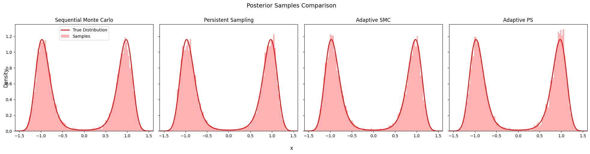
9. Posterior Comparison¶

Compare the posterior samples from all four algorithms.

# Calculate true distribution for plotting
x_linspace = jnp.linspace(-3, 3, 1000).reshape(-1, 1)
true_distribution = jnp.exp(log_posterior_fn(x_linspace))
true_distribution /= jnp.sum(true_distribution * (x_linspace[1] - x_linspace[0]))

fig, axes = plt.subplots(1, 4, figsize=(20, 5), sharey=True, sharex=True)

algorithms = [
    ("Sequential Monte Carlo", smc_final_state.particles, axes[0]),
    ("Persistent Sampling", ps_final_state.particles, axes[1]),
    ("Adaptive SMC", adaptive_smc_final_state.particles, axes[2]),
    ("Adaptive PS", adaptive_ps_final_state.particles, axes[3]),
]

for name, particles, ax in algorithms:
    ax.plot(
        x_linspace,
        true_distribution,
        color="red",
        lw=2,
        label="True Distribution",
    )

    ax.hist(
        particles[:, 0],
        bins=100,
        density=True,
        alpha=0.3,
        color="red",
        label="Samples",
    )
    ax.set_xlim(-1.6, 1.6)
    ax.set_title(f"{name}")

axes[0].legend()

fig.suptitle("Posterior Samples Comparison", fontsize=14, y=1.00)
fig.supxlabel("x", fontsize=12)
fig.supylabel("Density", fontsize=12)
fig.tight_layout()