In this example, we want to illustrate how to use the marginal sampler implementation mgrad_gaussian of the article Auxiliary gradient-based sampling algorithms Titsias & Papaspiliopoulos, 2018. We do so by using the simulated data from the example Gaussian Regression with the Elliptical Slice Sampler. Please also refer to the complementary example Bayesian Logistic Regression With Latent Gaussian Sampler.
Sampler Overview
In section we give a brief overview of the idea behind this particular sampler. For more details please refer to the original paper Auxiliary gradient-based sampling algorithms (here you can access the arXiv preprint).
Motivation: Auxiliary Metropolis-Hastings samplers
Let us recall how to sample from a target density using a Metropolis-Hasting sampler trough a marginal scheme process. The main idea is to have a mechanism that generate proposals which we then accept or reject according to a specific criterion. Concretely, suppose that we have an auxiliary scheme given by
Sample .
Generate proposal
Compute the Metropolis-Hasting ratio
Accept proposal with probability and reject it otherwise.
This scheme targets the auxiliary distribution in two steps.
Now, suppose we can instead compute the marginal proposal distribution in closed form, then an alternative scheme is given by:
We draw a proposal .
Then we compute the Metropolis-Hasting ratio
Accept proposal with probability and reject it otherwise.
Example: Auxiliary Metropolis-Adjusted Langevin Algorithm (MALA)
Let’s consider the case of an auxiliary random walk proposal for as in [Section 2.2] Auxiliary gradient-based sampling algorithms, it is shown that one can use a first order approximation to sample from the (intractable) density by choosing
The resulting marginal sampler can be shown to correspond to the Metropolis-adjusted Langevin algorithm (MALA) with
Latent Gaussian Models
A particular case of interest is the latent Gaussian model where the target density has the form
In this case, instead of linearising the full log density , we can linearise only, which, when combined with a random walk proposal , recovers to the following auxiliary proposal
where . The corresponding marginal density is
Sampling from , and therefore from , is done via Hastings-within-Gibbs as above.
A crucial point of this algorithm is the fact that can be precomputed and afterward modified cheaply when varies. This makes it easy to calibrate the step-size at low cost.
Now that we have a high-level understanding of the algorithm, let’s see how to use it in blackjax.
Notebook Cell
import matplotlib.pyplot as plt

plt.rcParams["axes.spines.right"] = False
plt.rcParams["axes.spines.top"] = False
import jax
from datetime import date
rng_key = jax.random.key(int(date.today().strftime("%Y%m%d")))import jax.numpy as jnp
import numpy as np
from blackjax import mgrad_gaussianWe generate data through a squared exponential kernel as in the example Gaussian Regression with the Elliptical Slice Sampler.
def squared_exponential(x, y, length, scale):
    dot_diff = jnp.dot(x, x) + jnp.dot(y, y) - 2 * jnp.dot(x, y)
    return scale**2 * jnp.exp(-0.5 * dot_diff / length**2)
n, d = 2000, 2
length, scale = 1.0, 1.0
y_sd = 1.0
# fake data
rng_key, kX, kf, ky = jax.random.split(rng_key, 4)
X = jax.random.uniform(kX, shape=(n, d))
Sigma = jax.vmap(
lambda x: jax.vmap(lambda y: squared_exponential(x, y, length, scale))(X)
)(X) + 1e-3 * jnp.eye(n)
invSigma = jnp.linalg.inv(Sigma)
f = jax.random.multivariate_normal(kf, jnp.zeros(n), Sigma)
y = f + jax.random.normal(ky, shape=(n,)) * y_sd
# conjugate results
posterior_cov = jnp.linalg.inv(invSigma + 1 / y_sd**2 * jnp.eye(n))
posterior_mean = jnp.dot(posterior_cov, y) * 1 / y_sd**2Let’s visualize the distribution of the vector y.
Source
plt.figure(figsize=(8, 5))
plt.hist(np.array(y), bins=50, density=True)
plt.xlabel("y")
plt.title("Histogram of data.")
plt.show()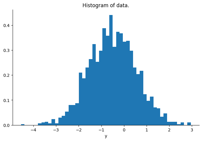
Sampling
Now we proceed to run the sampler. First, we set the sampler parameters:
# sampling parameters
n_warm = 2000
n_iter = 500
Next, we define the the log-probability function. For this we need to set the log-likelihood function.
loglikelihood_fn = lambda f: -0.5 * jnp.dot(y - f, y - f) / y_sd**2
logdensity_fn = lambda f: loglikelihood_fn(f) - 0.5 * jnp.dot(f @ invSigma, f)
Now we are ready to initialize the sampler. The output is type is a NamedTuple with the following fields:
init:
    A pure function which when called with the initial position and the
    target density probability function will return the kernel's initial
    state.

step:
    A pure function that takes a rng key, a state and possibly some
    parameters and returns a new state and some information about the
    transition.
init, kernel = mgrad_gaussian(
logdensity_fn=logdensity_fn, mean=jnp.zeros(n), covariance=Sigma, step_size=0.5
)We continue by setting the inference loop.
def inference_loop(rng, init_state, kernel, n_iter):
    keys = jax.random.split(rng, n_iter)

    def step(state, key):
        state, info = kernel(key, state)
        return state, (state, info)

    _, (states, info) = jax.lax.scan(step, init_state, keys)
    return states, info
We are now ready to run the sampler! The only extra parameters in the step function is delta, which (as seen in the sampler description) corresponds (in a loose sense) to the step-size of MALA algorithm.
%%time

initial_state = init(f)
rng_key, sample_key = jax.random.split(rng_key, 2)
states, info = inference_loop(sample_key, init(f), kernel, n_warm + n_iter)
samples = states.position[n_warm:]
CPU times: user 11.3 s, sys: 166 ms, total: 11.5 s
Wall time: 5.11 s
Diagnostics
Finally we evaluate the results.
error_mean = jnp.mean((samples.mean(axis=0) - posterior_mean) ** 2)
error_cov = jnp.mean((jnp.cov(samples, rowvar=False) - posterior_cov) ** 2)
print(
    f"Mean squared error for the mean vector {error_mean} and covariance matrix {error_cov}"
)
Mean squared error for the mean vector 0.003558369819074869 and covariance matrix 1.3298372323333751e-06
rng_key, sample_key = jax.random.split(rng_key, 2)
keys = jax.random.split(sample_key, 500)
predictive = jax.vmap(lambda k, f: f + jax.random.normal(k, (n,)) * y_sd)(
    keys, samples[-1000:]
)
Source
plt.figure(figsize=(8, 5))
plt.hist(np.array(y), bins=50, density=True)
plt.hist(np.array(predictive.reshape(-1)), bins=50, density=True, alpha=0.8)
plt.xlabel("y")
plt.title("Predictive distribution")
plt.show()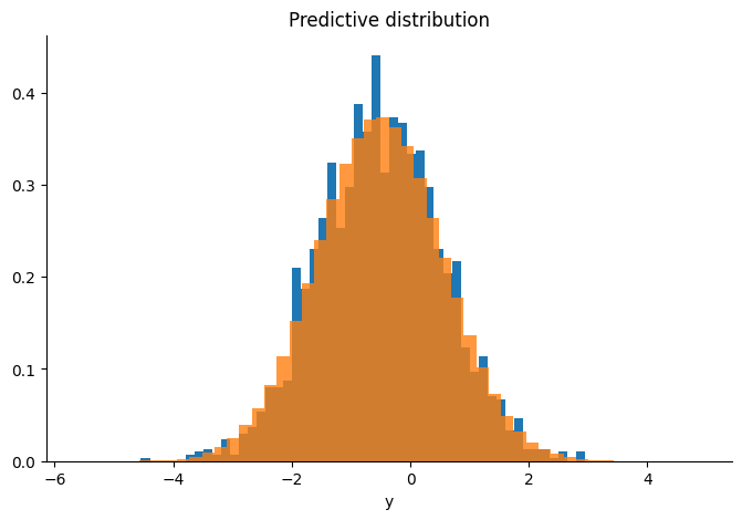
- Titsias, M. K., & Papaspiliopoulos, O. (2018). Auxiliary gradient-based sampling algorithms. Journal of the Royal Statistical Society: Series B (Statistical Methodology), 80(4), 749–767. https://doi.org/10.1111/rssb.12269