Code is based on This blog post by Thomas Wiecki (see Original PyMC3 Notebook). Converted to Blackjax by Aleyna Kara (@karalleyna) and Kevin Murphy (@murphyk). (For a Numpyro version, see here.)
We create T=18 different versions of the “two moons” dataset, each rotated by a different amount. These correspond to T different nonlinear binary classification “tasks” that we have to solve. We only get a few labeled samples from each each task, so solving them separately (with T independent MLPs, or multi layer perceptrons) will result in poor performance. If we pool all the data, and fit a single MLP, we also get poor performance, because we are mixing together different decision boundaries. But if we use a hierarchical Bayesian model, with one MLP per task, and one learned prior MLP, we will get better results, as we will see.
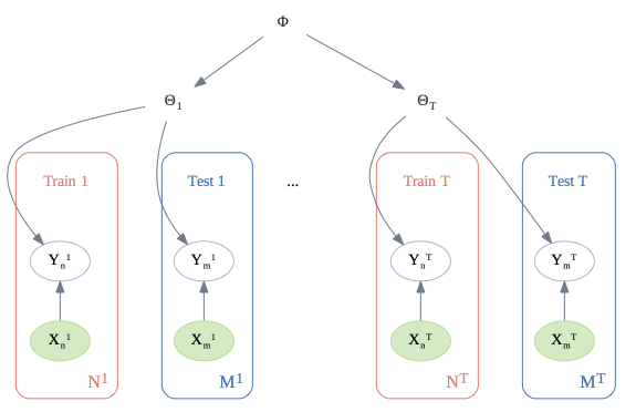
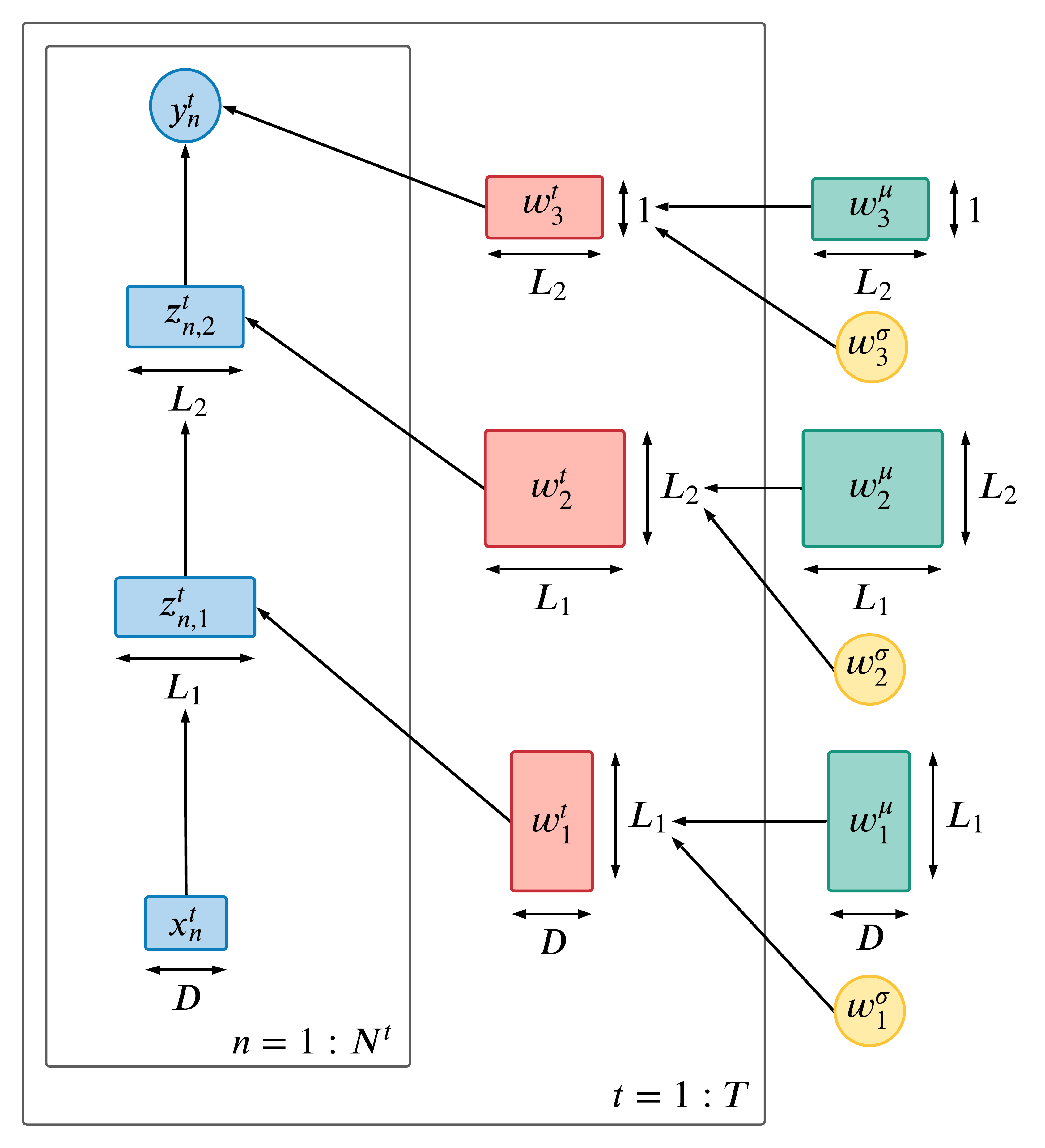
Below is a high level illustration of the multi-task setup. is the learned prior, and are the parameters for task . We assume training samples per task, and test samples. (We could of course consider more imbalanced scenarios.)
Setup
Notebook Cell
import matplotlib.pyplot as plt

plt.rcParams["axes.spines.right"] = False
plt.rcParams["axes.spines.top"] = False
import jax
from datetime import date
rng_key = jax.random.key(int(date.today().strftime("%Y%m%d")))from functools import partial
from warnings import filterwarnings
from flax import linen as nn
from flax.linen.initializers import ones
import jax.numpy as jnp
import numpy as np
import tensorflow_probability.substrates.jax.distributions as tfd
from sklearn.datasets import make_moons
from sklearn.preprocessing import scale
import blackjax
filterwarnings("ignore")import matplotlib as mpl
cmap = mpl.colormaps["coolwarm"]Data
We create T=18 different versions of the “two moons” dataset, each rotated by a different amount. These correspond to T different binary classification “tasks” that we have to solve.
Source
X, Y = make_moons(noise=0.3, n_samples=1000)
for i in range(2):
    plt.scatter(X[Y == i, 0], X[Y == i, 1], color=cmap(float(i)), label=f"Class {i}", alpha=.8)
plt.legend();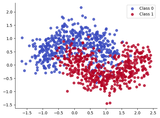
n_groups = 18

n_grps_sq = int(np.sqrt(n_groups))
n_samples = 100
def rotate(X, deg):
theta = np.radians(deg)
c, s = np.cos(theta), np.sin(theta)
R = np.matrix([[c, -s], [s, c]])
X = X.dot(R)
return np.asarray(X)np.random.seed(31)
Xs, Ys = [], []
for i in range(n_groups):
# Generate data with 2 classes that are not linearly separable
X, Y = make_moons(noise=0.3, n_samples=n_samples)
X = scale(X)
# Rotate the points randomly for each category
rotate_by = np.random.randn() * 90.0
X = rotate(X, rotate_by)
Xs.append(X)
Ys.append(Y)Xs = jnp.stack(Xs)
Ys = jnp.stack(Ys)
Xs_train = Xs[:, : n_samples // 2, :]
Xs_test = Xs[:, n_samples // 2 :, :]
Ys_train = Ys[:, : n_samples // 2]
Ys_test = Ys[:, n_samples // 2 :]Source
fig, axs = plt.subplots(
    figsize=(15, 12), nrows=n_grps_sq, ncols=n_grps_sq, sharex=True, sharey=True
)
axs = axs.flatten()
for i, (X, Y, ax) in enumerate(zip(Xs_train, Ys_train, axs)):
    for i in range(2):
        ax.scatter(X[Y == i, 0], X[Y == i, 1], color=cmap(float(i)), label=f"Class {i}", alpha=.8)

    ax.legend()
    ax.set(title=f"Category {i + 1}", xlabel="X1", ylabel="X2")


grid = jnp.mgrid[-3:3:100j, -3:3:100j].reshape((2, -1)).T
grid_3d = jnp.repeat(grid[None, ...], n_groups, axis=0)
plt.tight_layout();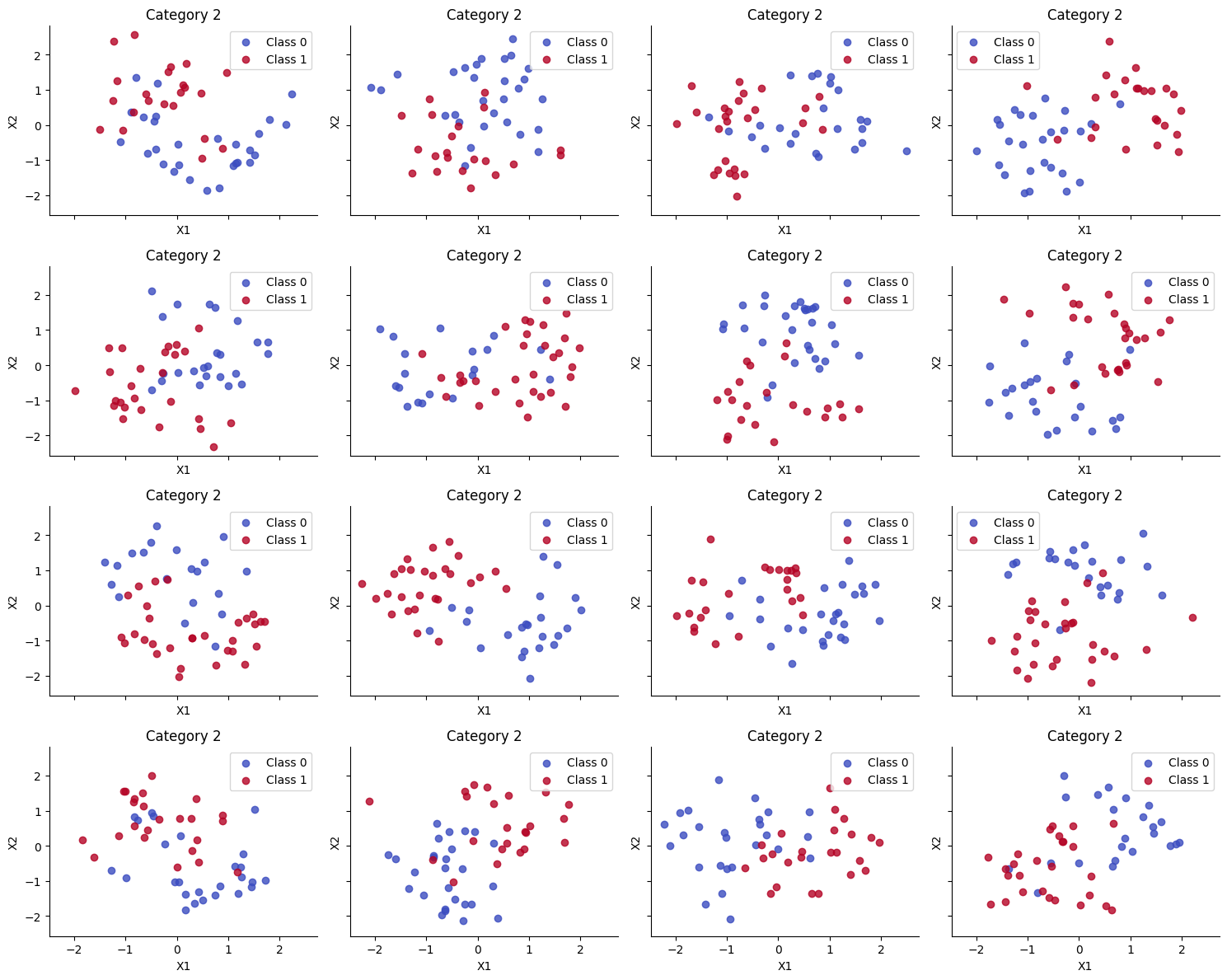
Utility Functions for Training and Testing
def inference_loop(rng_key, step_fn, initial_state, num_samples):
    def one_step(state, rng_key):
        state, _ = step_fn(rng_key, state)
        return state, state

    keys = jax.random.split(rng_key, num_samples)
    _, states = jax.lax.scan(one_step, initial_state, keys)

    return states
def get_predictions(model, samples, X, rng_key):
vectorized_apply = jax.vmap(model.apply, in_axes=(0, None), out_axes=0)
z = vectorized_apply(samples, X)
predictions = tfd.Bernoulli(logits=z).sample(seed=rng_key)
return predictions.squeeze(-1)def get_mean_predictions(predictions, threshold=0.5):
# compute mean prediction and confidence interval around median
mean_prediction = jnp.mean(predictions, axis=0)
return mean_prediction > thresholddef fit_and_eval(
rng_key,
model,
logdensity_fn,
X_train,
Y_train,
X_test,
grid,
n_groups=None,
num_warmup=1000,
num_samples=500,
):
(
init_key,
warmup_key,
inference_key,
train_key,
test_key,
grid_key,
) = jax.random.split(rng_key, 6)
if n_groups is None:
initial_position = model.init(init_key, jnp.ones(X_train.shape[-1]))
else:
initial_position = model.init(init_key, jnp.ones(X_train.shape))
# initialization
logprob = partial(logdensity_fn, X=X_train, Y=Y_train, model=model)
# warm up
adapt = blackjax.window_adaptation(blackjax.nuts, logprob)
(final_state, params), _ = adapt.run(warmup_key, initial_position, num_warmup)
step_fn = blackjax.nuts(logprob, **params).step
# inference
states = inference_loop(inference_key, step_fn, final_state, num_samples)
samples = states.position
# evaluation
predictions = get_predictions(model, samples, X_train, train_key)
Y_pred_train = get_mean_predictions(predictions)
predictions = get_predictions(model, samples, X_test, test_key)
Y_pred_test = get_mean_predictions(predictions)
pred_grid = get_predictions(model, samples, grid, grid_key)
return Y_pred_train, Y_pred_test, pred_gridHyperparameters
We use an MLP with 2 hidden layers, each with 5 hidden units.
# MLP params
hidden_layer_width = 5
n_hidden_layers = 2
Fit Separate MLPs, One Per Task
Let be the weight for node to node in layer in task . We assume
and compute the posterior for all the weights.
class NN(nn.Module):
    n_hidden_layers: int
    layer_width: int

    @nn.compact
    def __call__(self, x):
        for i in range(self.n_hidden_layers):
            x = nn.Dense(features=self.layer_width)(x)
            x = nn.tanh(x)
        return nn.Dense(features=1)(x)


bnn = NN(n_hidden_layers, hidden_layer_width)
def logprior_fn(params):
leaves, _ = jax.tree.flatten(params)
flat_params = jnp.concatenate([jnp.ravel(a) for a in leaves])
return jnp.sum(tfd.Normal(0, 1).log_prob(flat_params))
def loglikelihood_fn(params, X, Y, model):
logits = jnp.ravel(model.apply(params, X))
return jnp.sum(tfd.Bernoulli(logits).log_prob(Y))
def logdensity_fn_of_bnn(params, X, Y, model):
return logprior_fn(params) + loglikelihood_fn(params, X, Y, model)rng_key, eval_key = jax.random.split(rng_key)
keys = jax.random.split(eval_key, n_groups)
def fit_and_eval_single_mlp(key, X_train, Y_train, X_test):
return fit_and_eval(
key, bnn, logdensity_fn_of_bnn, X_train, Y_train, X_test, grid, n_groups=None
)
Ys_pred_train, Ys_pred_test, ppc_grid_single = jax.vmap(fit_and_eval_single_mlp)(
keys, Xs_train, Ys_train, Xs_test
)Results
Accuracy is reasonable, but the decision boundaries have not captured the underlying Z pattern in the data, due to having too little data per task. (Bayes model averaging results in a simple linear decision boundary, and prevents overfitting.)
Source
print(f"Train accuracy = {100 * jnp.mean(Ys_pred_train == Ys_train):.2f}%")Train accuracy = 86.78%
Source
print(f"Test accuracy = {100 * jnp.mean(Ys_pred_test == Ys_test):.2f}%")Test accuracy = 82.56%
Source
def plot_decision_surfaces_non_hierarchical(nrows=2, ncols=2):
    fig, axes = plt.subplots(
        figsize=(15, 12), nrows=nrows, ncols=ncols, sharex=True, sharey=True
    )
    axes = axes.flatten()
    for i, (X, Y_pred, Y_true, ax) in enumerate(
        zip(Xs_train, Ys_pred_train, Ys_train, axes)
    ):
        ax.contourf(
            grid[:, 0].reshape(100, 100),
            grid[:, 1].reshape(100, 100),
            ppc_grid_single[i, ...].mean(axis=0).reshape(100, 100),
            cmap=cmap,
        )
        for i in range(2):
            ax.scatter(
                X[Y_true == i, 0], X[Y_true == i, 1],
                color=cmap(float(i)), label=f"Class {i}", alpha=.8)
        ax.legend()
Below we show that the decision boundaries do not look reasonable, since there is not enough data to fit each model separately.
Source
plot_decision_surfaces_non_hierarchical(nrows=n_grps_sq, ncols=n_grps_sq)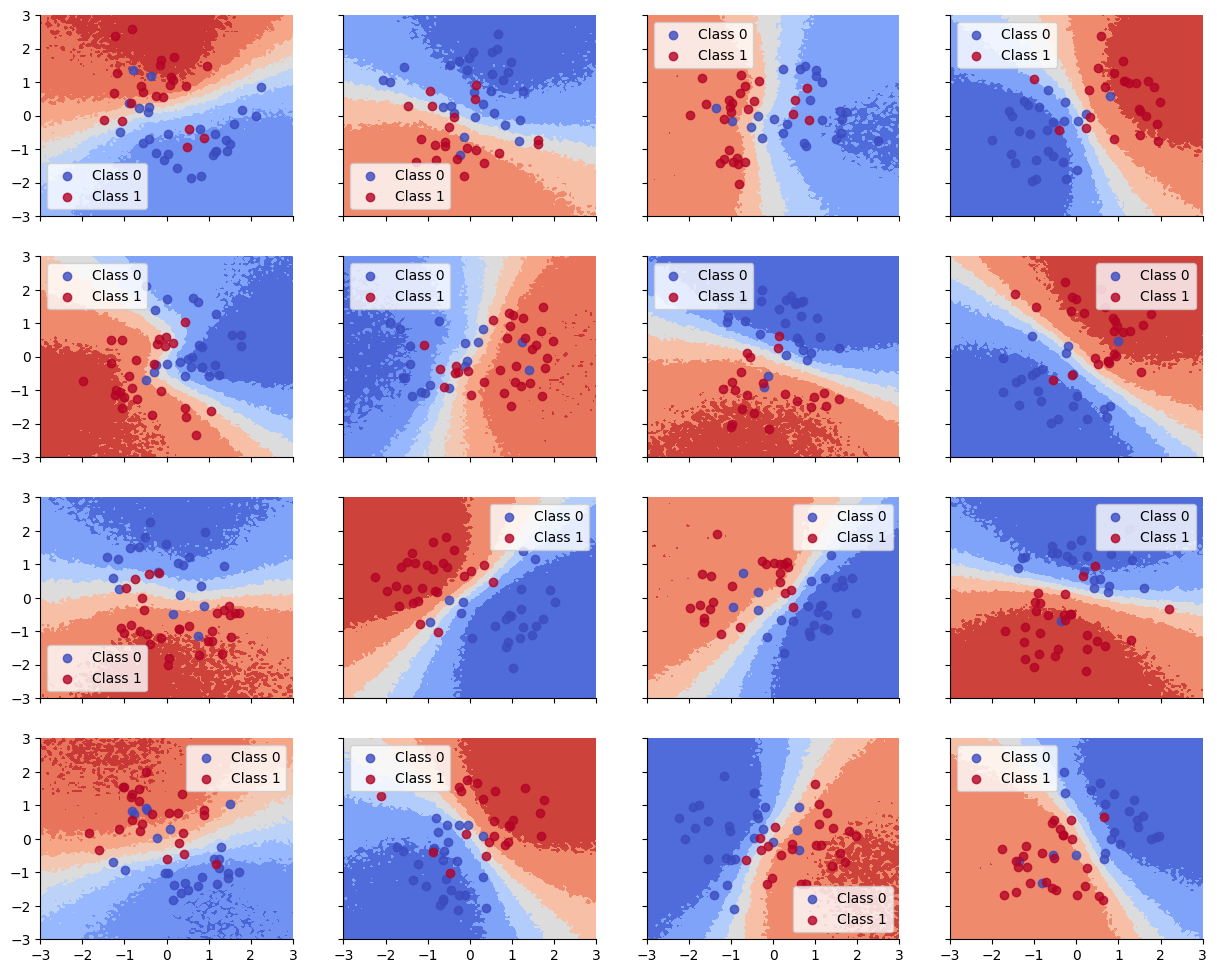
Source
plot_decision_surfaces_non_hierarchical()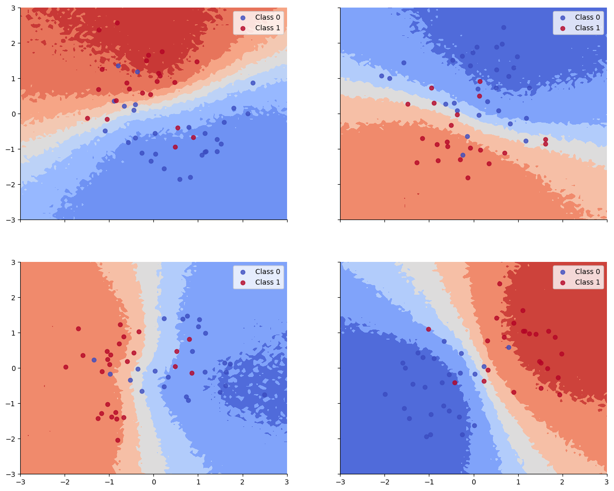
Hierarchical Model
Now we use a hierarchical Bayesian model, which has a common Gaussian prior for all the weights, but allows each task to have its own task-specific parameters. More precisely, let be the weight for node to node in layer in task . We assume
or, in non-centered form,
In the figure below, we illustrate this prior, using an MLP with D inputs, 2 hidden layers (of size and ), and a scalar output (representing the logit).
class NonCenteredDense(nn.Module):
    features: int

    @nn.compact
    def __call__(self, x):
        mu = self.param("mu", jax.random.normal, (x.shape[-1], self.features))
        eps = self.param(
            "eps", jax.random.normal, (n_groups, x.shape[-1], self.features)
        )
        std = self.param("std", ones, 1)
        w = mu + std * eps
        return x @ w


class HNN(nn.Module):
    n_hidden_layers: int
    layer_width: int

    @nn.compact
    def __call__(self, x):
        for i in range(self.n_hidden_layers):
            x = NonCenteredDense(features=self.layer_width)(x)
            x = nn.tanh(x)
        return nn.Dense(features=1)(x)


hnn = HNN(n_hidden_layers, hidden_layer_width)
def logprior_fn_of_hnn(params, model):
lp = 0
half_normal = tfd.HalfNormal(1.0)
for i in range(model.n_hidden_layers):
lparam = params["params"][f"NonCenteredDense_{i}"]
lp += tfd.Normal(0.0, 1.0).log_prob(lparam["mu"]).sum()
lp += tfd.Normal(0.0, 1.0).log_prob(lparam["eps"]).sum()
lp += half_normal.log_prob(lparam["std"]).sum()
lp += logprior_fn(params["params"]["Dense_0"])
return lp
def loglikelihood_fn(params, X, Y, model):
logits = jnp.ravel(model.apply(params, X))
return jnp.sum(tfd.Bernoulli(logits).log_prob(jnp.ravel(Y)))
def logdensity_fn_of_hnn(params, X, Y, model):
return logprior_fn_of_hnn(params, model) + loglikelihood_fn(params, X, Y, model)%%time
rng_key, inference_key = jax.random.split(rng_key)
Ys_hierarchical_pred_train, Ys_hierarchical_pred_test, ppc_grid = fit_and_eval(
inference_key,
hnn,
logdensity_fn_of_hnn,
Xs_train,
Ys_train,
Xs_test,
grid_3d,
n_groups=n_groups,
)CPU times: user 2min 17s, sys: 795 ms, total: 2min 18s
Wall time: 2min 5s
Results
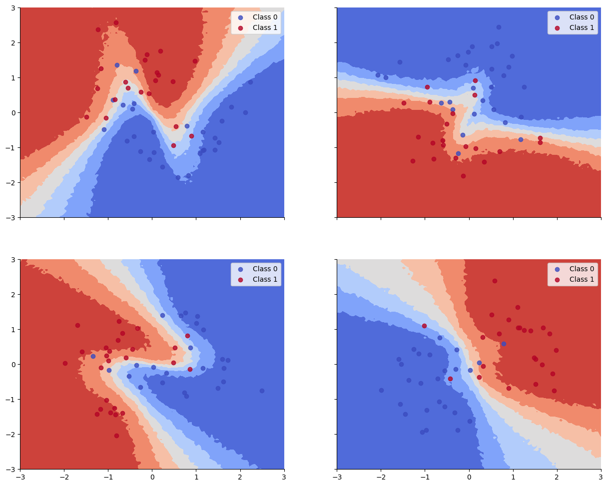
We see that the train and test accuracy are higher, and the decision boundaries all have the shared “Z” shape, as desired.
Source
print(
    "Train accuracy = {:.2f}%".format(
        100 * jnp.mean(Ys_hierarchical_pred_train == Ys_train)
    )
)
Train accuracy = 90.89%
Source
print(
    "Test accuracy = {:.2f}%".format(
        100 * jnp.mean(Ys_hierarchical_pred_test == Ys_test)
    )
)
Test accuracy = 87.11%
def plot_decision_surfaces_hierarchical(nrows=2, ncols=2):
    fig, axes = plt.subplots(
        figsize=(15, 12), nrows=nrows, ncols=ncols, sharex=True, sharey=True
    )

    for i, (X, Y_pred, Y_true, ax) in enumerate(
        zip(Xs_train, Ys_hierarchical_pred_train, Ys_train, axes.flatten())
    ):
        ax.contourf(
            grid[:, 0].reshape((100, 100)),
            grid[:, 1].reshape((100, 100)),
            ppc_grid[:, i, :].mean(axis=0).reshape(100, 100),
            cmap=cmap,
        )
        for i in range(2):
            ax.scatter(
                X[Y_true == i, 0], X[Y_true == i, 1],
                color=cmap(float(i)), label=f"Class {i}", alpha=.8)
        ax.legend()
Source
plot_decision_surfaces_hierarchical(nrows=n_grps_sq, ncols=n_grps_sq)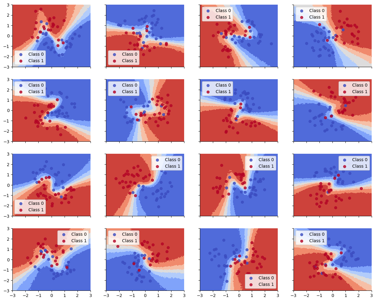
Source
plot_decision_surfaces_hierarchical()