Regime switching Hidden Markov model

This example replicates the case study analyzing financial time series, specifically the daily difference in log price data of Google’s stock, referred to as returns $r_t$ .

We’ll assume that at any given time $t$ the stock’s returns will follow one of two regimes: an independent random walk regime where $r_t \sim \mathcal{N}(\alpha_1, \sigma^2_1)$ and an autoregressive regime where $r_t \sim \mathcal{N}(\alpha_2 + \rho r_{t-1}, \sigma_2^2)$ . Being on either of the two regimes, $s_t\in \{0, 1\}$ , will depend on the previous time’s regime $s_{t-1}$ , call these probabilities $p_{s_{t-1}, s_{t}}$ for $s_{t-1}, s_t \in \{0, 1\}$ . Set as parameters of the model $p_{1,1}$ and $p_{2,2}$ and define the complementary probabilities by definition: $p_{1,2} = 1-p_{1,1}$ and $p_{2,1} = 1-p_{2,2}$ . Since the regime at any time is unobserved, we instead carry over time the probability of belonging to either one regime as $\xi_{1t} + \xi_{2t} = 1$ . Finally, we need to model initial values, both for returns $r_0$ and probability of belonging to one of the two regimes $\xi_{10}$ .

In the whole, our regime-switching model is defined by the likelihood

\begin{split} L(\mathbf{r}|\alpha, \rho, \sigma^2, \mathbf{p}, r_0, \xi_{10}) &= \prod_t \xi_{1t}\eta_{1t} + (1-\xi_{1t})\eta_{2t} \\ \xi_{1t} &= \frac{\xi_{1t-1}\eta_{1t}}{\xi_{1t-1}\eta_{1t} + (1-\xi_{1t-1})\eta_{2t}}, \end{split}

(1)

where $\eta_{jt} = p_{j,1}$ , $\mathcal{N}(r_t;\alpha_1, \sigma_1^2) + p_{j,2}$ , and $\mathcal{N}(r_t; \alpha_2 + \rho r_{t-1}, \sigma_2^2)$ for $j\in\{0, 1\}$ . And the priors of the parameters are:

\begin{split} \alpha_1, \alpha_2 &\sim \mathcal{N}(0, 0.1) \\ \rho &\sim \mathcal{N}^0(1, 0.1) \\ \sigma_1, \sigma_2 &\sim \mathcal{C}^+(1) \\ p_{1,1}, p_{2,2} &\sim \mathcal{Beta}(10, 2) \\ r_0 &\sim \mathcal{N}(0, 0.1) \\ \xi_{10} &\sim \mathcal{Beta}(2, 2), \end{split}

(2)

where $\mathcal{N}^0$ indicates the truncated at 0 Gaussian distribution and $\mathcal{C}^+$ the half-Cauchy distribution.

import jax

jax.config.update("jax_enable_x64", True)

from datetime import date
rng_key = jax.random.key(int(date.today().strftime("%Y%m%d")))

import jax.numpy as jnp
import numpy as np
import numpyro
import numpyro.distributions as distrib
import pandas as pd
from jax.scipy.stats import norm
from numpyro.diagnostics import print_summary
from numpyro.infer.util import initialize_model

import blackjax


class RegimeMixtureDistribution(distrib.Distribution):
    arg_constraints = {
        "alpha": distrib.constraints.real,
        "rho": distrib.constraints.positive,
        "sigma": distrib.constraints.positive,
        "p": distrib.constraints.interval(0, 1),
        "xi_0": distrib.constraints.interval(0, 1),
        "y_0": distrib.constraints.real,
        "T": distrib.constraints.positive_integer,
    }
    support = distrib.constraints.real

    def __init__(self, alpha, rho, sigma, p, xi_0, y_0, T, validate_args=True):
        self.alpha, self.rho, self.sigma, self.p, self.xi_0, self.y_0, self.T = (
            alpha,
            rho,
            sigma,
            p,
            xi_0,
            y_0,
            T,
        )
        super().__init__(event_shape=(T,), validate_args=validate_args)

    def log_prob(self, value):
        def obs_t(carry, y):
            y_prev, log_xi = carry  # log_xi: [log P(s_{t-1}=1), log P(s_{t-1}=2)]
            log_eta_1 = norm.logpdf(y, loc=self.alpha[0], scale=self.sigma[0])
            log_eta_2 = norm.logpdf(
                y, loc=self.alpha[1] + y_prev * self.rho, scale=self.sigma[1]
            )
            # log P(y_t | s_{t-1} = j) for j in {1, 2}
            log_lik_1 = jnp.logaddexp(
                jnp.log(self.p[0]) + log_eta_1,
                jnp.log1p(-self.p[0]) + log_eta_2,
            )
            log_lik_2 = jnp.logaddexp(
                jnp.log1p(-self.p[1]) + log_eta_1,
                jnp.log(self.p[1]) + log_eta_2,
            )
            log_liks = jnp.array([log_lik_1, log_lik_2])
            log_xi_unnorm = log_xi + log_liks
            log_lik_total = jax.nn.logsumexp(log_xi_unnorm)
            new_log_xi = log_xi_unnorm - log_lik_total
            return (y, new_log_xi), log_lik_total

        log_xi_0 = jnp.log(jnp.array([self.xi_0, 1.0 - self.xi_0]))
        _, log_liks = jax.lax.scan(obs_t, (self.y_0, log_xi_0), value)
        return jnp.sum(log_liks)

    def sample(self, key, sample_shape=()):
        return jnp.zeros(sample_shape + self.event_shape)


class RegimeSwitchHMM:
    def __init__(self, T, y) -> None:
        self.T = T
        self.y = y

    def model(self, y=None):
        rho = numpyro.sample("rho", distrib.TruncatedNormal(1.0, 0.1, low=0.0))
        alpha = numpyro.sample("alpha", distrib.Normal(0.0, 0.1).expand([2]))
        sigma = numpyro.sample("sigma", distrib.HalfCauchy(1.0).expand([2]))
        p = numpyro.sample("p", distrib.Beta(10.0, 2.0).expand([2]))
        xi_0 = numpyro.sample("xi_0", distrib.Beta(2.0, 2.0))
        y_0 = numpyro.sample("y_0", distrib.Normal(0.0, 0.1))

        numpyro.sample(
            "obs",
            RegimeMixtureDistribution(alpha, rho, sigma, p, xi_0, y_0, self.T),
            obs=y,
        )

    def initialize_model(self, rng_key, n_chain):
        (init_params, *_), self.potential_fn, *_ = initialize_model(
            rng_key,
            self.model,
            model_kwargs={"y": self.y},
            dynamic_args=True,
        )
        # Separate the two regimes by anchoring sigma at [3, 10] in constrained
        # space (numpyro uses log transform, so unconstrained = log(constrained)).
        # Without this, chains near sigma[0] ≈ sigma[1] can fall into degenerate
        # modes where one regime becomes inactive.
        init_params = dict(init_params)
        init_params["sigma"] = jnp.log(jnp.array([3.0, 10.0]))
        init_params["rho"] = jnp.zeros(())  # log(1) = 0, the prior mode
        flat, unravel_fn = jax.flatten_util.ravel_pytree(init_params)
        kchain = jax.random.split(rng_key, n_chain)
        self.init_params = jax.vmap(
            lambda k: unravel_fn(flat + 0.1 * jax.random.normal(k, flat.shape))
        )(kchain)

    def logdensity_fn(self, params):
        return -self.potential_fn(self.y)(params)


def inference_loop(rng, init_state, kernel, n_iter):
    keys = jax.random.split(rng, n_iter)

    def step(state, key):
        state, info = kernel(key, state)
        return state, (state, info)

    _, (states, info) = jax.lax.scan(step, init_state, keys)
    return states, info

/opt/hostedtoolcache/Python/3.13.12/x64/lib/python3.13/site-packages/tqdm/auto.py:21: TqdmWarning: IProgress not found. Please update jupyter and ipywidgets. See https://ipywidgets.readthedocs.io/en/stable/user_install.html
  from .autonotebook import tqdm as notebook_tqdm

url = "https://raw.githubusercontent.com/blackjax-devs/blackjax/main/docs/examples/data/google.csv"
data = pd.read_csv(url)
y = data["dl_ac"].values * 100
T, _ = data.shape

dist = RegimeSwitchHMM(T, y)

n_chain, n_warm, n_iter = 8, 2000, 2000
ksam, kinit = jax.random.split(jax.random.key(0), 2)
dist.initialize_model(kinit, n_chain)

tic1 = pd.Timestamp.now()
k_warm, k_sample = jax.random.split(ksam)

(_, parameters), _ = blackjax.window_adaptation(
    blackjax.nuts, dist.logdensity_fn
).run(k_warm, jax.tree.map(lambda x: x[0], dist.init_params), n_warm)

kernel = blackjax.nuts(dist.logdensity_fn, **parameters).step


def one_chain(k_sam, init_param):
    init_state = blackjax.nuts(dist.logdensity_fn, **parameters).init(init_param)
    state, info = inference_loop(k_sam, init_state, kernel, n_iter)
    return state.position, info


k_sample = jax.random.split(k_sample, n_chain)
samples, infos = jax.vmap(one_chain)(k_sample, dist.init_params)
tic2 = pd.Timestamp.now()
print("Runtime for NUTS", tic2 - tic1)

Runtime for NUTS 0 days 00:01:18.045767

print_summary(samples)


                mean       std    median      5.0%     95.0%     n_eff     r_hat
  alpha[0]      0.06      0.08      0.06     -0.08      0.20  27827.21      1.00
  alpha[1]      0.01      0.10      0.01     -0.15      0.18  26813.28      1.00
      p[0]      2.71      0.42      2.69      2.05      3.37   6837.55      1.00
      p[1]      1.82      0.91      1.75      0.46      3.26  10453.65      1.00
       rho     -0.02      0.11     -0.01     -0.18      0.16  26029.82      1.00
  sigma[0]      1.04      0.05      1.04      0.97      1.12  21694.94      1.00
  sigma[1]      2.16      0.18      2.14      1.85      2.44  16638.53      1.00
      xi_0      0.50      1.04      0.47     -1.18      2.24  25371.45      1.00
       y_0      0.00      0.10      0.00     -0.16      0.17  25656.75      1.00

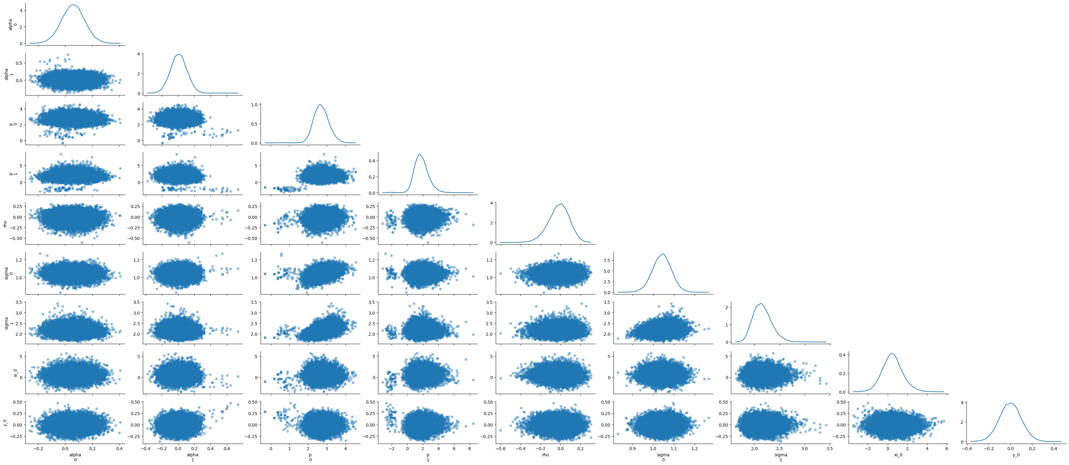
idata = az.from_dict({"posterior": samples})
az.plot_pair(idata, marginal=True, marginal_kind='kde')
plt.tight_layout();