Parameter estimation in ODE models with a probabilistic ODE solver

This tutorial explains how to estimate unknown parameters of initial value problems (IVPs) using probabilistic solvers as provided by ProbDiffEq in combination with Markov Chain Monte Carlo (MCMC) methods from BlackJAX.

TL;DR¶

Compute log-posterior of IVP parameters given observations of the IVP solution with ProbDiffEq. Sample from this posterior using BlackJAX. Evaluating the log-likelihood of the data is described in this paper Tronarp et al., 2022. Based on this log-likelihood, sampling from the log-posterior is as done in this paper Kersting et al., 2020.

Technical setup¶

Let $f$ be a known vector field. In this example, we use the Lotka-Volterra model. (We get our IVP implementations from DiffEqZoo.) Consider an ordinary differential equation

\dot y(t) = f(y(t)), \quad 0 \leq t \leq T

(1)

subject to an unknown initial condition $y(0) = \theta$ . The probabilistic IVP solution is an approximation of the posterior distribution (e.g. Eq. (12) in Krämer et al., 2022)

p\left(y ~|~ [\dot y(t_n) = f(y(t_n))]_{n=0}^N, y(0) = \theta\right)

(2)

for a Gaussian process prior over $y$ and a pre-determined or adaptively selected grid $t_0, ..., t_N$ .

We don’t know the initial condition of the IVP, but assume that we have noisy observations of the IVP solution $y$ at the terminal time $T$ of the integration problem,

p(\text{data}~|~ y(T)) = N(y(T), \sigma^2 I)

(3)

for some $\sigma > 0$ . We can use these observations to reconstruct $\theta$ , for example by sampling from $p(\theta ~|~ \text{data}) \propto p(\text{data}~|~\theta)p(\theta)$ (which is a function of $\theta$ ).

Now, one way of evaluating this posterior is to use any numerical solver, for example a Runge-Kutta method, to approximate $y(T)$ from $\theta$ and evaluate $N(y(T), \sigma^2 I)$ to get $p(\text{data} ~|~ \theta)$ (the $p(\theta)$ component is known). But this ignores a few crucial concepts (e.g., the numerical error of the approximation; we refer to the references linked above). We can use a probabilistic solver instead of “any” numerical solver and build a more comprehensive model:

We can combine probabilistic IVP solvers with MCMC methods to estimate $\theta$ from $\text{data}$ in a way that quantifies numerical approximation errors (and other model mismatches). To do so, we approximate the distribution of the IVP solution given the parameter $p(y(T) \mid \theta)$ and evaluate the marginal distribution of $N(y(T), \sigma^2I)$ given the probabilistic IVP solution. More formally, we use ProbDiffEq to evaluate the density of the unnormalised posterior

M(\theta) := p(\theta \mid \text{data})\propto p(\text{data} \mid \theta)p(\theta)

(4)

where “ $\propto$ ” means “proportional to” and the likelihood stems from the IVP solution

p(\text{data} \mid \theta) = \int p(\text{data} \mid y(T)) p(y(T) \mid [\dot y(t_n) = f(y(t_n))]_{n=0}^N, y(0) = \theta), \theta) d y(T)

(5)

Loosely speaking, this distribution averages $N(y(T), \sigma^2I)$ over all IVP solutions $y(T)$ that are realistic given the differential equation, grid $t_0, ..., t_N$ , and prior distribution $p(y)$ . This is useful, because if the approximation error is large, $M(\theta)$ “knows this”. If the approximation error is ridiculously small, $M(\theta)$ “knows this” too and we recover the procedure described for non-probabilistic solvers above. Interestingly, non-probabilistic solvers cannot do this averaging because they do not yield a statistical description of estimated IVP solutions. Non-probabilistic solvers would also fail if the observations were noise-free (i.e. $\sigma = 0$ ), but the present example notebook remains stable. (Try it yourself!)

To sample $\theta$ according to $M$ (respectively $\log M$ ), we evaluate $M(\theta)$ with ProbDiffEq, compute its gradient with JAX, and use this gradient to sample $\theta$ with BlackJAX:

ProbDiffEq: Compute the probabilistic IVP solution by approximating $p(y(T) ~|~ [\dot y(t_n) = f(y(t_n))]_n, y(0) = \theta)$
ProbDiffEq: Evaluate $M(\theta)$ by marginalising over the IVP solution computed in step 1.
JAX: Compute the gradient $\nabla_\theta M(\theta)$
BlackJAX: Sample from $\log M(\theta)$ using, for example, the No-U-Turn-Sampler (which requires $\nabla_\theta M(\theta))$ .

Here is how:

import jax
from jax import config

# x64 precision
config.update("jax_enable_x64", True)

# CPU
config.update("jax_platform_name", "cpu")

from datetime import date
rng_key = jax.random.key(int(date.today().strftime("%Y%m%d")))

import functools

import blackjax
import jax
import jax.numpy as jnp
from diffeqzoo import backend, ivps
from probdiffeq import ivpsolve, ivpsolvers, stats, taylor

# IVP examples in JAX
if not backend.has_been_selected:
    backend.select("jax")

Problem setting¶

First, we set up an IVP and create some artificial data by simulating the system with “incorrect” initial conditions.

f, u0, (t0, t1), f_args = ivps.lotka_volterra()


@jax.jit
def vf(y, *, t, p=()):
    # diffeqzoo Lotka-Volterra signature: f(y, a, b, c, d) — no explicit t
    return f(y, *f_args)


theta_true = u0 + 0.5 * jnp.flip(u0)
theta_guess = u0  # initial guess


# Build the SSM once (shape determined by theta; values don't matter).
_ref_tcoeffs = taylor.odejet_padded_scan(
    lambda y: vf(y, t=t0, p=()), (theta_guess,), num=2
)
_, _ref_ibm, ssm = ivpsolvers.prior_wiener_integrated(
    _ref_tcoeffs, ssm_fact="dense", output_scale=10.0
)


def _make_solver(theta, *, strategy_fn):
    """Build a probdiffeq solver initialised at *theta*, reusing the shared SSM."""
    tcoeffs = taylor.odejet_padded_scan(
        lambda y: vf(y, t=t0, p=()), (theta,), num=2
    )
    init_cond, ibm, _ = ivpsolvers.prior_wiener_integrated(
        tcoeffs, ssm_fact="dense", output_scale=10.0
    )
    ts0 = ivpsolvers.correction_ts0(vf, ssm=ssm)
    strategy = strategy_fn(ssm=ssm)
    solver = ivpsolvers.solver(strategy, correction=ts0, prior=ibm, ssm=ssm)
    return init_cond, solver

def plot_solution(sol, *, ax, marker=".", **plotting_kwargs):
    # sol.u is a list of Taylor-coefficient arrays; sol.u[0] holds the trajectory.
    traj = sol.u[0]  # shape (n_times, 2)
    for d in [0, 1]:
        ax.plot(sol.t, traj[:, d], marker="None", **plotting_kwargs)
        ax.plot(sol.t[0], traj[0, d], marker=marker, **plotting_kwargs)
        ax.plot(sol.t[-1], traj[-1, d], marker=marker, **plotting_kwargs)
    return ax


@jax.jit
def solve_adaptive(theta, *, save_at):
    # Use a filter strategy for visualisation (smoother is not compatible with save_at)
    init_cond, solver = _make_solver(theta, strategy_fn=ivpsolvers.strategy_filter)
    adaptive_solver = ivpsolvers.adaptive(solver, ssm=ssm)
    return ivpsolve.solve_adaptive_save_at(
        init_cond, save_at=save_at, adaptive_solver=adaptive_solver, dt0=0.1, ssm=ssm
    )


save_at = jnp.linspace(t0, t1, num=250, endpoint=True)
solve_save_at = functools.partial(solve_adaptive, save_at=save_at)

# Visualise the initial guess and the data

fig, ax = plt.subplots()

data_kwargs = {"alpha": 0.5, "color": "gray"}
ax.annotate("Data", (13.0, 30.0), **data_kwargs)
solution = solve_save_at(theta_true)
ax = plot_solution(solution, ax=ax, **data_kwargs)

guess_kwargs = {"color": "C3"}
ax.annotate("Initial guess", (7.5, 20.0), **guess_kwargs)
solution = solve_save_at(theta_guess)
ax = plot_solution(solution, ax=ax, **guess_kwargs)
plt.show()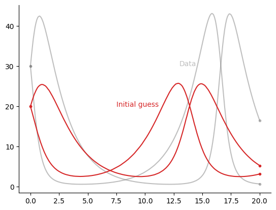

Log-posterior densities via ProbDiffEq¶

Set up a log-posterior density function that we can plug into BlackJAX. Choose a Gaussian prior centered at the initial guess with a large variance.

mean = theta_guess
cov = jnp.eye(2) * 30  # fairly uninformed prior

# Fixed-grid solve for reverse-mode differentiability.
# Uses a smoother strategy, required by log_marginal_likelihood_terminal_values.
@jax.jit
def solve_fixed(theta, *, ts):
    init_cond, solver = _make_solver(theta, strategy_fn=ivpsolvers.strategy_smoother)
    return ivpsolve.solve_fixed_grid(init_cond, grid=ts, solver=solver, ssm=ssm)


@jax.jit
def logposterior_fn(theta, *, data, ts, obs_stdev=0.1):
    sol = solve_fixed(theta, ts=ts)
    terminal = stats.markov_select_terminal(sol.posterior)
    log_lik = stats.log_marginal_likelihood_terminal_values(
        data, standard_deviation=obs_stdev, posterior=terminal, ssm=ssm
    )
    log_prior = jax.scipy.stats.multivariate_normal.logpdf(theta, mean=mean, cov=cov)
    return log_lik + log_prior


ts = jnp.linspace(t0, t1, endpoint=True, num=100)
data = solve_fixed(theta_true, ts=ts).u[0][-1]  # terminal state, shape (2,)

log_M = functools.partial(logposterior_fn, data=data, ts=ts)

print(jnp.exp(log_M(theta_true)), ">=", jnp.exp(log_M(theta_guess)), "?")

0.002049860936172054 >= 0.0 ?

Sampling with BlackJAX¶

From here on, BlackJAX takes over:

Set up a sampler.

@functools.partial(jax.jit, static_argnames=["kernel", "num_samples"])
def inference_loop(rng_key, kernel, initial_state, num_samples):
    def one_step(state, rng_key):
        state, _ = kernel(rng_key, state)
        return state, state

    keys = jax.random.split(rng_key, num_samples)
    _, states = jax.lax.scan(one_step, initial_state, keys)

    return states

Initialise the sampler, warm it up, and run the inference loop.

initial_position = theta_guess

# WARMUP
warmup = blackjax.window_adaptation(
    blackjax.nuts, log_M, progress_bar=True
)

rng_key, warmup_key = jax.random.split(rng_key)
(initial_state, tuned_parameters), _ = warmup.run(
    warmup_key, initial_position, num_steps=200)

Running window adaptation

# INFERENCE LOOP
rng_key, sample_key = jax.random.split(rng_key)
nuts_kernel = blackjax.nuts(log_M, **tuned_parameters).step
states = inference_loop(
    sample_key, kernel=nuts_kernel, initial_state=initial_state, num_samples=150
)

Visualisation¶

Now that we have samples of $\theta$ , let’s plot the corresponding solutions:

solution_samples = jax.vmap(solve_save_at)(states.position)

# Visualise the initial guess and the data
# vmap returns a single batched IVPSolution; iterate by index.

fig, ax = plt.subplots()

sample_kwargs = {"color": "C0"}
ax.annotate("Samples", (2.75, 31.0), **sample_kwargs)
for i in range(solution_samples.u[0].shape[0]):
    sol_i = jax.tree.map(lambda x: x[i], solution_samples)
    ax = plot_solution(sol_i, ax=ax, linewidth=0.1, alpha=0.75, **sample_kwargs)

data_kwargs = {"color": "gray"}
ax.annotate("Data", (18.25, 40.0), **data_kwargs)
solution = solve_save_at(theta_true)
ax = plot_solution(solution, ax=ax, linewidth=4, alpha=0.5, **data_kwargs)

guess_kwargs = {"color": "gray"}
ax.annotate("Initial guess", (6.0, 12.0), **guess_kwargs)
solution = solve_save_at(theta_guess)
ax = plot_solution(solution, ax=ax, linestyle="dashed", alpha=0.75, **guess_kwargs)
plt.show()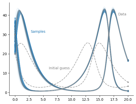

The samples cover a perhaps surprisingly large range of potential initial conditions, but lead to the “correct” data.

In parameter space, this is what it looks like:

plt.title("Posterior samples (parameter space)")
plt.plot(states.position[:, 0], states.position[:, 1], "o", alpha=0.5, markersize=4)
plt.plot(theta_true[0], theta_true[1], "P", label="Truth", markersize=8)
plt.plot(theta_guess[0], theta_guess[1], "P", label="Initial guess", markersize=8)
plt.legend()
plt.show()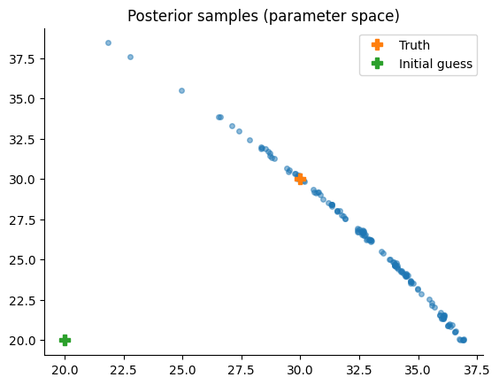

Let’s add the value of $M$ to the plot to see whether the sampler covers the entire region of interest.

xlim = 18, jnp.amax(states.position[:, 0]) + 0.5
ylim = 18, jnp.amax(states.position[:, 1]) + 0.5

xs = jnp.linspace(*xlim, num=300)
ys = jnp.linspace(*ylim, num=300)
Xs, Ys = jnp.meshgrid(xs, ys)

Thetas = jnp.stack((Xs, Ys))
log_M_vmapped_x = jax.vmap(log_M, in_axes=-1, out_axes=-1)
log_M_vmapped = jax.vmap(log_M_vmapped_x, in_axes=-1, out_axes=-1)
Zs = log_M_vmapped(Thetas)

fig, ax = plt.subplots(ncols=2, sharex=True, sharey=True)

ax_samples, ax_heatmap = ax

fig.suptitle("Posterior samples (parameter space)")
ax_samples.plot(
    states.position[:, 0], states.position[:, 1], ".", alpha=0.5, markersize=4
)
ax_samples.plot(theta_true[0], theta_true[1], "P", label="Truth", markersize=8)
ax_samples.plot(
    theta_guess[0], theta_guess[1], "P", label="Initial guess", markersize=8
)
ax_samples.legend()
im = ax_heatmap.contourf(Xs, Ys, jnp.exp(Zs), cmap="cividis", alpha=0.8)
plt.colorbar(im)
plt.show()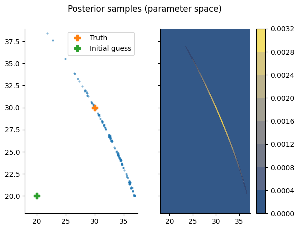

Looks great!

Conclusion¶

In conclusion, a log-posterior density function can be provided by ProbDiffEq such that any of BlackJAX’ samplers yield parameter estimates of IVPs.

What’s next¶

Try to get a feeling for how the sampler reacts to changing observation noises, solver parameters, and so on. We could extend the sampling problem from $\theta \mapsto \log M(\theta)$ to some $(\theta, \sigma) \mapsto \log \tilde M(\theta, \sigma)$ , i.e., treat the observation noise as unknown and run Hamiltonian Monte Carlo in a higher-dimensional parameter space. We could also add a more suitable prior distribution $p(\theta)$ to regularise the problem.

A final side note: We could also replace the sampler with an optimisation algorithm and use this procedure to solve boundary value problems (albeit this may not be very efficient; use this algorithm instead Krämer & Hennig, 2021).

References¶

Tronarp, F., Bosch, N., & Hennig, P. (2022). Fenrir: Physics-Enhanced Regression for Initial Value Problems. International Conference on Machine Learning, 21776–21794.
Kersting, H., Krämer, N., Schiegg, M., Daniel, C., Tiemann, M., & Hennig, P. (2020). Differentiable Likelihoods for Fast Inversion of “Likelihood-Free” Dynamical Systems. International Conference on Machine Learning, 5198–5208.
Krämer, N., Bosch, N., Schmidt, J., & Hennig, P. (2022). Probabilistic ODE Solutions in Millions of Dimensions. International Conference on Machine Learning, 11634–11649.
Krämer, N., & Hennig, P. (2021). Linear-Time Probabilistic Solutions of Boundary Value Problems. Advances in Neural Information Processing Systems, 34, 11160–11171.