Use with Numpyro models

Blackjax accepts any log-probability function as long as it is compatible with JAX’s primitive. In this notebook we show how we can use Numpyro as a modeling language together with Blackjax as an inference library.

Before you start

You will need Numpyro to run this example. Please follow the installation instructions on Numpyro’s repository.

We reproduce the Eight Schools example from the Numpyro documentation (all credit for the model goes to the Numpyro team).

Show code cell content Hide code cell content

import numpy as np


J = 8
y = np.array([28.0, 8.0, -3.0, 7.0, -1.0, 1.0, 18.0, 12.0])
sigma = np.array([15.0, 10.0, 16.0, 11.0, 9.0, 11.0, 10.0, 18.0])

import jax

from datetime import date
rng_key = jax.random.key(int(date.today().strftime("%Y%m%d")))

We implement the non-centered version of the hierarchical model:

import numpyro
import numpyro.distributions as dist
from numpyro.infer.reparam import TransformReparam


def eight_schools_noncentered(J, sigma, y=None):
    mu = numpyro.sample("mu", dist.Normal(0, 5))
    tau = numpyro.sample("tau", dist.HalfCauchy(5))
    with numpyro.plate("J", J):
        with numpyro.handlers.reparam(config={"theta": TransformReparam()}):
            theta = numpyro.sample(
                "theta",
                dist.TransformedDistribution(
                    dist.Normal(0.0, 1.0), dist.transforms.AffineTransform(mu, tau)
                ),
            )
        numpyro.sample("obs", dist.Normal(theta, sigma), obs=y)

Warning

The model applies a transformation to the theta variable. As a result, the samples generated by Blackjax will be samples in the transformed space and you will have to transform them back to the original space with Numpyro.

We need to translate the model into a log-probability function that will be used by Blackjax to perform inference. For that we use the initialize_model function in Numpyro’s internals. We will also use the initial position it returns to initialize the inference:

from numpyro.infer.util import initialize_model

rng_key, init_key = jax.random.split(rng_key)
init_params, potential_fn_gen, *_ = initialize_model(
    init_key,
    eight_schools_noncentered,
    model_args=(J, sigma, y),
    dynamic_args=True,
)

Numpyro return a potential function, which is easily transformed back into a logdensity function that is required by Blackjax:

logdensity_fn = lambda position: -potential_fn_gen(J, sigma, y)(position)
initial_position = init_params.z

We can now run the window adaptation for the NUTS sampler:

import blackjax

num_warmup = 2000

adapt = blackjax.window_adaptation(
    blackjax.nuts, logdensity_fn, target_acceptance_rate=0.8
)
rng_key, warmup_key = jax.random.split(rng_key)
(last_state, parameters), _ = adapt.run(warmup_key, initial_position, num_warmup)
kernel = blackjax.nuts(logdensity_fn, **parameters).step

Let us now perform inference with the tuned kernel:

Show code cell content Hide code cell content

def inference_loop(rng_key, kernel, initial_state, num_samples):
    @jax.jit
    def one_step(state, rng_key):
        state, info = kernel(rng_key, state)
        return state, (state, info)

    keys = jax.random.split(rng_key, num_samples)
    _, (states, infos) = jax.lax.scan(one_step, initial_state, keys)

    return states, (
        infos.acceptance_rate,
        infos.is_divergent,
        infos.num_integration_steps,
    )

num_sample = 1000
rng_key, sample_key = jax.random.split(rng_key)
states, infos = inference_loop(sample_key, kernel, last_state, num_sample)
_ = states.position["mu"].block_until_ready()

To make sure that the model sampled correctly, let’s compute the average acceptance rate and the number of divergences:

Show code cell content Hide code cell content

acceptance_rate = np.mean(infos[0])
num_divergent = np.mean(infos[1])

print(f"\Average acceptance rate: {acceptance_rate:.2f}")
print(f"There were {100*num_divergent:.2f}% divergent transitions")

\Average acceptance rate: 0.93
There were 0.00% divergent transitions

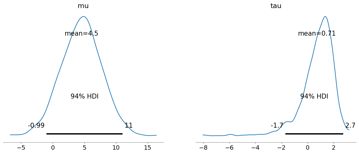
Finally let us now plot the distribution of the parameters. Note that since we use a transformed variable, Numpyro does not output the school treatment effect directly:

import matplotlib.pyplot as plt
import arviz as az

idata = az.from_dict(posterior={k: v[None, ...] for k, v in states.position.items()})

az.plot_posterior(idata, var_names=["mu", "tau"]);

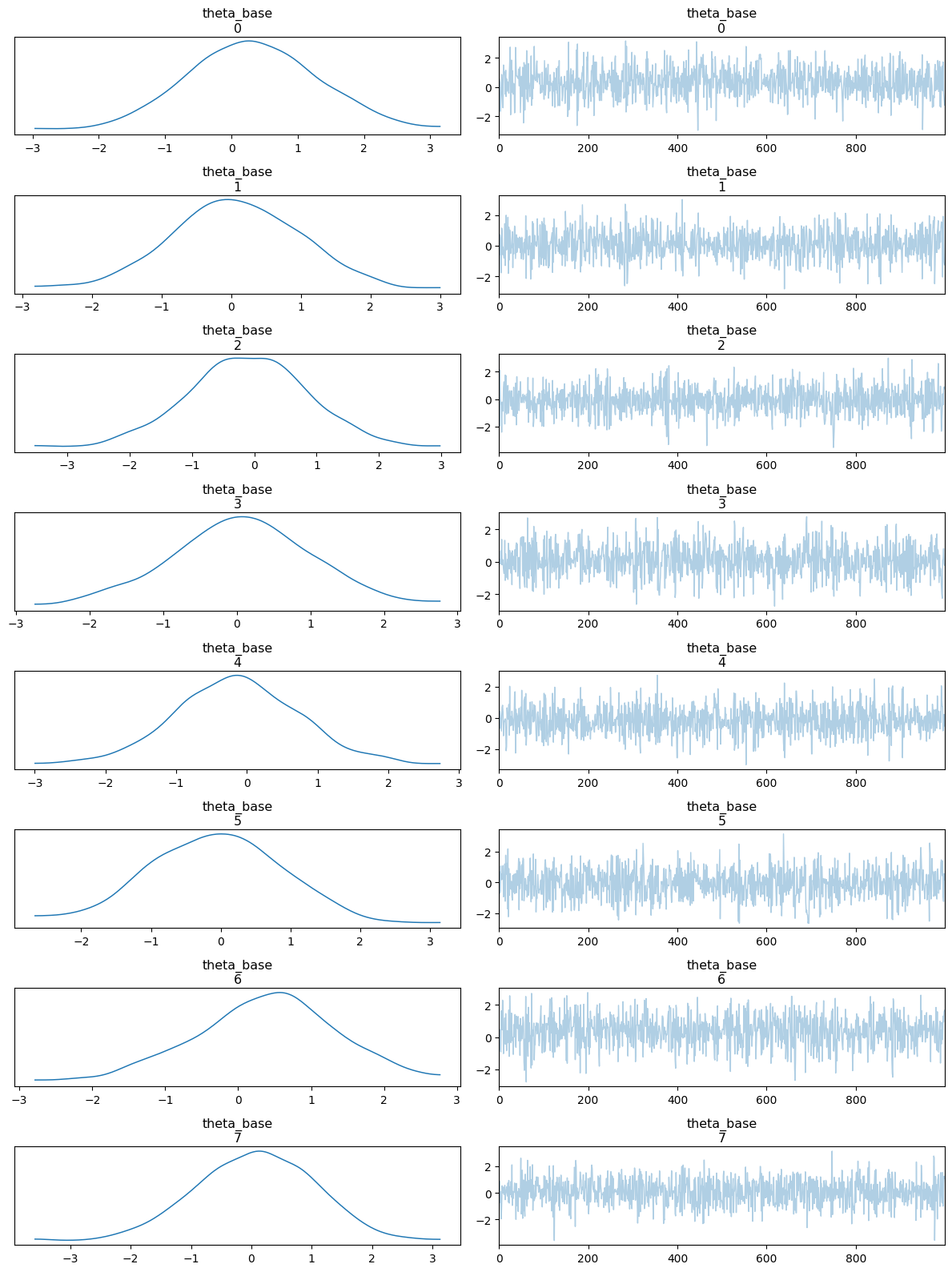
az.plot_trace(idata, var_names=["theta_base"], compact=False)
plt.tight_layout();

Show code cell source Hide code cell source

for i in range(J):
    print(
        f"Relative treatment effect for school {i}: {np.mean(idata.posterior['theta_base'][:, i]):.2f}"
    )

Relative treatment effect for school 0: 0.31
Relative treatment effect for school 1: 0.56
Relative treatment effect for school 2: 0.07
Relative treatment effect for school 3: -0.11
Relative treatment effect for school 4: 0.60
Relative treatment effect for school 5: 0.47
Relative treatment effect for school 6: 0.23
Relative treatment effect for school 7: -0.16