A Quick Introduction to Blackjax

BlackJAX is an MCMC sampling library based on JAX. BlackJAX provides well-tested and ready to use sampling algorithms. It is also explicitly designed to be modular: it is easy for advanced users to mix-and-match different metrics, integrators, trajectory integrations, etc.

In this notebook we provide a simple example based on basic Hamiltonian Monte Carlo and the NUTS algorithm to showcase the architecture and interfaces in the library

import matplotlib.pyplot as plt
import numpy as np

import jax
import jax.numpy as jnp
import jax.scipy.stats as stats

import blackjax

from datetime import date
rng_key = jax.random.key(int(date.today().strftime("%Y%m%d")))

The Problem

We’ll generate observations from a normal distribution of known loc and scale to see if we can recover the parameters in sampling. MCMC algorithms usually assume samples are being drawn from an unconstrained Euclidean space. Hence why we’ll log transform the scale parameter, so that sampling is done on the real line. Samples can be transformed back to their original space in post-processing. Let’s take a decent-size dataset with 1,000 points:

loc, scale = 10, 20
observed = np.random.normal(loc, scale, size=1_000)

def logdensity_fn(loc, log_scale, observed=observed):
    """Univariate Normal"""
    scale = jnp.exp(log_scale)
    logpdf = stats.norm.logpdf(observed, loc, scale)
    return jnp.sum(logpdf)


logdensity = lambda x: logdensity_fn(**x)

HMC

Sampler Parameters

inv_mass_matrix = np.array([0.5, 0.01])
num_integration_steps = 60
step_size = 1e-3

hmc = blackjax.hmc(logdensity, step_size, inv_mass_matrix, num_integration_steps)

Set the Initial State

The initial state of the HMC algorithm requires not only an initial position, but also the potential energy and gradient of the potential energy at this position (for example, in the context of Bayesian modeling, the output of the log posterior function evaluated at the initial position). BlackJAX provides a new_state function to initialize the state from an initial position.

initial_position = {"loc": 1.0, "log_scale": 1.0}
initial_state = hmc.init(initial_position)
initial_state

HMCState(position={'loc': 1.0, 'log_scale': 1.0}, logdensity=Array(-32966.492, dtype=float32), logdensity_grad={'loc': Array(1199.4308, dtype=float32, weak_type=True), 'log_scale': Array(61095.113, dtype=float32, weak_type=True)})

Build the Kernel and Inference Loop

The HMC kernel is easy to obtain:

hmc_kernel = jax.jit(hmc.step)

BlackJAX does not provide a default inference loop, but it easy to implement with JAX’s lax.scan:

def inference_loop(rng_key, kernel, initial_state, num_samples):
    @jax.jit
    def one_step(state, rng_key):
        state, _ = kernel(rng_key, state)
        return state, state

    keys = jax.random.split(rng_key, num_samples)
    _, states = jax.lax.scan(one_step, initial_state, keys)

    return states

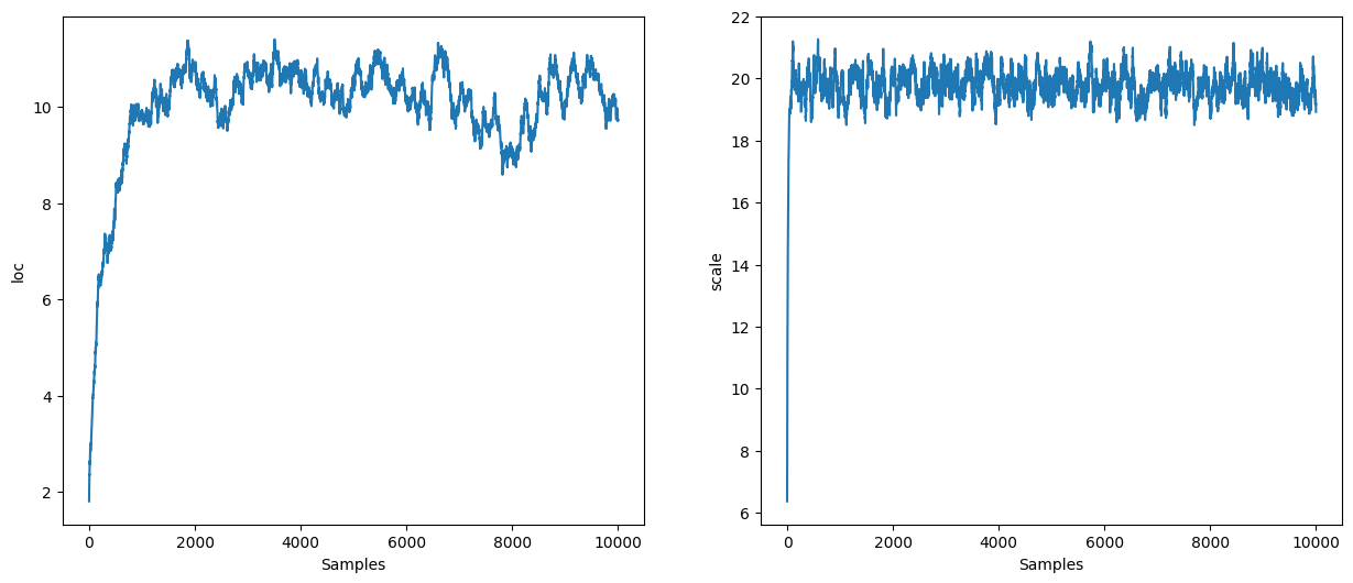
Inference

%%time
rng_key, sample_key = jax.random.split(rng_key)
states = inference_loop(sample_key, hmc_kernel, initial_state, 10_000)

mcmc_samples = states.position
mcmc_samples["scale"] = jnp.exp(mcmc_samples["log_scale"]).block_until_ready()

CPU times: user 1.4 s, sys: 23.7 ms, total: 1.42 s
Wall time: 1.42 s

Show code cell source Hide code cell source

fig, (ax, ax1) = plt.subplots(ncols=2, figsize=(15, 6))
ax.plot(mcmc_samples["loc"])
ax.set_xlabel("Samples")
ax.set_ylabel("loc")

ax1.plot(mcmc_samples["scale"])
ax1.set_xlabel("Samples")
ax1.set_ylabel("scale");

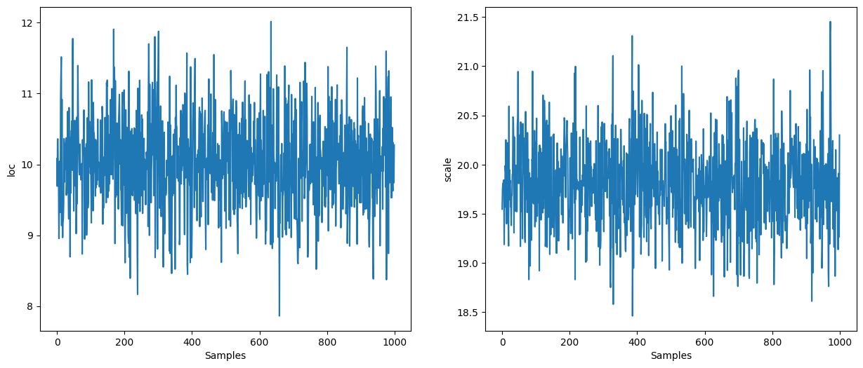
NUTS

NUTS is a dynamic algorithm: the number of integration steps is determined at runtime. We still need to specify a step size and a mass matrix:

inv_mass_matrix = np.array([0.5, 0.01])
step_size = 1e-3

nuts = blackjax.nuts(logdensity, step_size, inv_mass_matrix)

initial_position = {"loc": 1.0, "log_scale": 1.0}
initial_state = nuts.init(initial_position)
initial_state

HMCState(position={'loc': 1.0, 'log_scale': 1.0}, logdensity=Array(-32966.492, dtype=float32), logdensity_grad={'loc': Array(1199.4308, dtype=float32, weak_type=True), 'log_scale': Array(61095.113, dtype=float32, weak_type=True)})

%%time
rng_key, sample_key = jax.random.split(rng_key)
states = inference_loop(sample_key, nuts.step, initial_state, 4_000)

mcmc_samples = states.position
mcmc_samples["scale"] = jnp.exp(mcmc_samples["log_scale"]).block_until_ready()

CPU times: user 6.53 s, sys: 71.5 ms, total: 6.6 s
Wall time: 6.59 s

Show code cell source Hide code cell source

fig, (ax, ax1) = plt.subplots(ncols=2, figsize=(15, 6))
ax.plot(mcmc_samples["loc"])
ax.set_xlabel("Samples")
ax.set_ylabel("loc")

ax1.plot(mcmc_samples["scale"])
ax1.set_xlabel("Samples")
ax1.set_ylabel("scale");

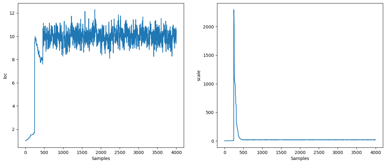
Use Stan’s Window Adaptation

Specifying the step size and inverse mass matrix is cumbersome. We can use Stan’s window adaptation to get reasonable values for them so we have, in practice, no parameter to specify.

The adaptation algorithm takes a function that returns a transition kernel given a step size and an inverse mass matrix:

%%time

warmup = blackjax.window_adaptation(blackjax.nuts, logdensity)
rng_key, warmup_key, sample_key = jax.random.split(rng_key, 3)
(state, parameters), _ = warmup.run(warmup_key, initial_position, num_steps=1000)

CPU times: user 1.42 s, sys: 88.7 ms, total: 1.51 s
Wall time: 1.49 s

We can use the obtained parameters to define a new kernel. Note that we do not have to use the same kernel that was used for the adaptation:

%%time

kernel = blackjax.nuts(logdensity, **parameters).step
states = inference_loop(sample_key, kernel, state, 1_000)

mcmc_samples = states.position
mcmc_samples["scale"] = jnp.exp(mcmc_samples["log_scale"]).block_until_ready()

CPU times: user 1.05 s, sys: 60.5 ms, total: 1.11 s
Wall time: 1.1 s

Show code cell source Hide code cell source

fig, (ax, ax1) = plt.subplots(ncols=2, figsize=(15, 6))
ax.plot(mcmc_samples["loc"])
ax.set_xlabel("Samples")
ax.set_ylabel("loc")

ax1.plot(mcmc_samples["scale"])
ax1.set_xlabel("Samples")
ax1.set_ylabel("scale");