Nested Sampling

The tempered SMC chapter showed that multimodal targets defeat energy-based samplers such as HMC and NUTS: escaping one potential well requires a rare, high-energy excursion, so a single chain stays trapped in whichever mode it started in. Particle methods can mitigate this, and nested sampling Skilling, 2006 is a distinctive and popular member of the family. Particle methods are also useful for estimating the marginal likelihood — the central quantity nested sampling was originally conceived to compute,

Rather than tempering the likelihood, nested sampling maintains a population of live particles drawn from the prior and repeatedly replaces the worst (lowest-likelihood) ones with a fresh prior draw constrained to lie above the discarded likelihood value. It shares much of its machinery with SMC, but takes a different path: instead of interpolating from prior to posterior by geometry or temperature, it walks a sequence of constrained priors $\pi^*$, indexed by a likelihood threshold $L^*$ that ratchets upward from $-\infty$ (the constraint is vacuous and $\pi^*$ is just the prior) toward the likelihood peak ($\pi^*$ collapses onto the dominant mode). Because that threshold is set by the live particles themselves, the path is adaptive by construction. Nested sampling is also usually implemented with procedures that tune the inner MCMC kernel from the particle cloud of the previous iteration; in this respect it is natural to compare against inner kernel tuning, which exploits the same mechanism.

In this notebook we use blackjax.nss, the Nested Slice Sampling implementation of Yallup et al., 2026, which pairs the generic nested-sampling outer loop with a hit-and-run slice sampler as the inner kernel. That pairing — a generic outer loop plus a pluggable inner kernel — is one instance of the broader blackjax.ns primitives available for building samplers, and we return to them in the synthesis.

The implementation follows the library’s standard init / step construction and acts on a particle cloud much as SMC does; we flag the choices unique to nested sampling as they arise.

This chapter demonstrates:

1. A Bimodal Target (Multimodality) — nested sampling and adaptive tempered SMC both populate the two modes from the prior and agree on the evidence; on this target the two are interchangeable.

2. A Phase Transition — a sharp spike holding 90% of the evidence makes the target a first-order phase transition: nested sampling compresses straight through it in prior volume, posing a stiff challenge for tempering approaches.

import matplotlib.pyplot as plt

plt.rcParams["axes.spines.right"] = False
plt.rcParams["axes.spines.top"] = False

import jax
import jax.numpy as jnp
import numpy as np
from jax.scipy.stats import multivariate_normal
from jax.scipy.special import logsumexp

import blackjax
from blackjax.ns.utils import finalise, log_weights, ess
from blackjax.ns.utils import sample as ns_sample

# adaptive tempered SMC with inner-kernel tuning, for the comparison throughout
from blackjax import adaptive_tempered_smc
from blackjax.smc import resampling, extend_params
from blackjax.smc.inner_kernel_tuning import as_top_level_api as inner_kernel_tuning
from blackjax.smc.tuning.from_particles import particles_covariance_matrix
from blackjax.mcmc import random_walk

rng_key = jax.random.key(42)

Section 1: A Bimodal Target (Multimodality)¶

We inherit the example problem and SMC setup from tempered SMC: a prior $p_0(x) = \mathcal{N}(x \mid 0, 1)$ and a log-likelihood $\ln\mathcal{L}(x) = -5\,(x^2 - 1)^2$. The algorithm consumes JAX functions defining a logprior_fn and a loglikelihood_fn,

def loglikelihood_fn(x):
    return -5 * jnp.square(jnp.sum(x**2, axis=-1) - 1)


def logprior_fn(x):
    d = x.shape[-1]
    return multivariate_normal.logpdf(x, jnp.zeros((d,)), jnp.eye(d))

The likelihood peaks on the ring $\sum_i x_i^2 = 1$; in one dimension that is the pair of modes at $x = \pm 1$. Because the $\mathcal{N}(0, 1)$ prior comfortably covers both, the initial live set — drawn straight from the prior — populates both modes from the outset. So far this mirrors the SMC setup exactly.

Running Nested Sampling¶

blackjax.nss follows the usual BlackJAX init / step pattern. The two algorithm choices worth understanding are:

• num_delete — how many of the lowest-likelihood live points are replaced per step. Together with num_live this fixes the volume compression per step, and hence the size of the outer move, playing a role similar to target_ess in adaptive SMC. Here each step keeps 90% of the live set (num_delete / num_live = 0.1), matching the SMC target ESS of 0.9.

• num_inner_steps — how many constrained slice moves generate each replacement point. The new point must decorrelate from the one it replaces, so a useful rule of thumb is to scale num_inner_steps with the dimension, of order max(5, 2*dim).

num_live = 1000
num_delete = 100

algo = blackjax.nss(
    logprior_fn=logprior_fn,
    loglikelihood_fn=loglikelihood_fn,
    num_inner_steps=5,
    num_delete=num_delete,
)

Adaptive tempered SMC steps until its temperature $\beta$ reaches 1; nested sampling has no such landmark and simply compresses until enough of the evidence has been collected. state.integrator keeps the running totals that make that judgement — logZ accumulated from the dead points and logZ_live, the optimistic contribution still held by the live set — and the standard rule stops once the live set holds a negligible share: $\log Z_\text{live} - \log Z < -3$ Skilling, 2006, the dlogz default below.

def nested_sampling_loop(rng_key, algo, initial_particles, dlogz=-3.0):
    """Run nested sampling until the live points hold a negligible share of Z."""
    state = algo.init(initial_particles)
    step = jax.jit(algo.step)

    dead = []
    while True:
        rng_key, subkey = jax.random.split(rng_key)
        state, info = step(subkey, state)
        dead.append(info)

        if state.integrator.logZ_live - state.integrator.logZ < dlogz:
            break

    return finalise(state, dead)

The live points are initialised by sampling the prior directly, then we run the loop. The finalise utility stitches the dead points together with the final live set into a single NSInfo. Its particles carry, for every sample, the position, the loglikelihood, and the loglikelihood_birth (the contour level at which the point was born) — everything needed to assign importance weights after the fact.

%%time

rng_key, init_key, run_key = jax.random.split(rng_key, 3)
initial_particles = jax.random.normal(init_key, (num_live, 1))

ns_run = nested_sampling_loop(run_key, algo, initial_particles)
print("Number of dead points:", ns_run.particles.loglikelihood.shape[0])

Number of dead points: 5400
CPU times: user 6.49 s, sys: 304 ms, total: 6.79 s
Wall time: 3.38 s

With the run finalised, blackjax.ns.utils turns that bag of dead points into the quantities we actually want. Each carries an importance weight $w_i \propto \mathcal{L}_i\,\mathrm{d}X_i$ — its likelihood times the sliver of prior volume $\mathrm{d}X_i$ that its shell swept out. The volumes $X_i$ are not known exactly but follow a known stochastic law Skilling, 2006, so log_weights returns not one weight per point but shape independent simulations of the whole volume sequence — which is what lets every downstream quantity come with an error bar for free.

rng_key, w_key = jax.random.split(rng_key)

# Each dead point i carries log w_i = log L_i + log dX_i; the volumes are stochastic,
# so log_weights draws `shape` independent volume sequences (the columns).
logw = log_weights(w_key, ns_run, shape=200)          # (num_dead, 200)

# Evidence: sum the weights down the points, once per sequence -> mean and a free error bar.
logZ = logsumexp(logw, axis=0)
print(f"log Z = {logZ.mean():.3f} +/- {logZ.std():.3f}")

# The weights are very uneven, so the raw dead-point count overstates the information held.
# ess reports the equivalent number of equally-weighted posterior draws.
print(f"effective sample size = {ess(w_key, ns_run):.0f}"
      f"  (from {ns_run.particles.loglikelihood.shape[0]} dead points)")

log Z = -1.565 +/- 0.035

effective sample size = 3184  (from 5400 dead points)

Particle Methods mitigate energy barriers¶

We built the importance weights above; sample (blackjax.ns.utils.sample) closes the loop, resampling the dead points by those weights — log_weights followed by a draw with replacement — into the equally-weighted posterior draws we plot.

rng_key, sample_key = jax.random.split(rng_key)
posterior = ns_sample(sample_key, ns_run, 4000).position[:, 0]

A single nested-sampling run recovers both modes with the correct relative weight — exactly where HMC and NUTS got stuck.

We use adaptive tempered SMC for comparison: a random-walk Metropolis inner kernel whose proposal covariance is tuned from the particle population at every temperature (the inner-kernel tuning of the preamble, with the optimal $2.38^2/d$ scaling), summing the per-temperature normalising constants for $\log Z$.

def adaptive_smc(rng_key, logprior_fn, loglikelihood_fn, initial_particles,
                 num_mcmc_steps, target_ess=0.9):
    """Adaptive tempered SMC with a random-walk kernel tuned from the particles."""
    d = initial_particles.shape[-1]
    rmh_kernel = random_walk.build_rmh()

    def rwmh_step(key, state, logdensity, cov):
        move = lambda k, x: jax.random.multivariate_normal(k, x, cov)
        return rmh_kernel(key, state, logdensity, move)

    def tune_from_particles(key, state, info):  # ITK: cloud at step i sets step i+1
        cov = jnp.atleast_2d(particles_covariance_matrix(state.particles))
        return extend_params({"cov": (2.38**2 / d) * cov})

    smc = inner_kernel_tuning(
        logprior_fn=logprior_fn,
        loglikelihood_fn=loglikelihood_fn,
        mcmc_step_fn=rwmh_step,
        mcmc_init_fn=random_walk.init,
        resampling_fn=resampling.systematic,
        smc_algorithm=adaptive_tempered_smc,
        mcmc_parameter_update_fn=tune_from_particles,
        initial_parameter_value=extend_params({"cov": jnp.eye(d)}),
        target_ess=target_ess,
        num_mcmc_steps=num_mcmc_steps,
    )

    loglike_v = jax.vmap(loglikelihood_fn)
    state = smc.init(initial_particles)
    step = jax.jit(smc.step)
    logZ = 0.0
    mean_logL = []                    # E[logL] of the ensemble at each temperature step
    while state.sampler_state.tempering_param < 1:  # run until temperature reaches 1
        rng_key, subkey = jax.random.split(rng_key)
        state, info = step(subkey, state)
        logZ += info.log_likelihood_increment
        mean_logL.append(loglike_v(state.sampler_state.particles).mean())
    return logZ, state.sampler_state.particles, jnp.array(mean_logL)

%%time

rng_key, smc_init_key, smc_key = jax.random.split(rng_key, 3)
smc_particles = jax.random.normal(smc_init_key, (5000, 1))
logZ_smc, smc_post, _ = adaptive_smc(
    smc_key, logprior_fn, loglikelihood_fn, smc_particles, num_mcmc_steps=10
)
print(f"tempered SMC log Z = {logZ_smc:.3f}")

tempered SMC log Z = -1.556
CPU times: user 5.53 s, sys: 103 ms, total: 5.63 s
Wall time: 1.94 s

Both particle methods recover both modes, and agree on the evidence ($\log Z \approx -1.5$). On this target they are interchangeable; the next section finds one where they are not.

Source

linspace = jnp.linspace(-2, 2, 2000)[:, None]
density = jnp.exp(loglikelihood_fn(linspace) + logprior_fn(linspace))
density /= jnp.sum(density) * (linspace[1, 0] - linspace[0, 0])

fig, ax = plt.subplots()
ax.hist(np.array(posterior), bins=80, density=True, histtype="step", lw=1.5, label="nested sampling")
ax.hist(np.array(smc_post[:, 0]), bins=80, density=True, histtype="step", lw=1.5, label="tempered SMC")
ax.plot(np.array(linspace[:, 0]), np.array(density), "k", lw=1, label="true density")
ax.legend()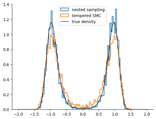

Section 2: A Phase Transition¶

The bimodal target was easy enough that tempered SMC matched nested sampling. The classical example that separates them has a phase transition — the regime nested sampling is built for. We demonstrate it with a simple mixture of Gaussians with exaggerated features, though physical systems routinely exhibit such transitions (a liquid boiling, a ferromagnet magnetising). Along the path from prior to posterior the probability mass can jump discontinuously between regions, leaving a band of intermediate distributions that hold almost no mass — the sampling analogue of latent heat. We will show that nested sampling, marching by prior volume, contracts straight through it.

Our target is a $D = 10$ likelihood under a flat prior on $[-5, 5]^{10}$: a broad Gaussian background ($\sigma = 1$) plus a narrow spike ($\sigma = 0.1$) at the origin. Evidence is height $\times$ volume, and the spike’s volume is only $(0.1/1)^{10} = 10^{-10}$ of the background’s; to make the transition sharp we scale the spike tall enough ($h \approx 9\times10^{10}$) that it still carries ~90% of $Z$. Resolving that spike is the whole challenge.

D = 10
box_low, box_high = -5.0, 5.0
log_box_volume = D * jnp.log(box_high - box_low)

means = jnp.zeros((2, D))
sigmas = jnp.array([1.0, 0.1])       # broad background, narrow spike
heights = jnp.array([1.0, 9e10])     # spike ~9e10 taller, so it holds ~90% of Z


def loglikelihood_mix(x):
    sq_dist = jnp.sum((x - means) ** 2, axis=-1)
    return logsumexp(jnp.log(heights) - sq_dist / (2 * sigmas**2))


def logprior_mix(x):
    inside = jnp.all((x >= box_low) & (x <= box_high))
    return jnp.where(inside, -log_box_volume, -jnp.inf)

The same height-times-volume accounting gives the analytic evidence to check against — a logsumexp over the two components, minus the log box volume — and confirms the split:

# each Gaussian bump integrates to h * (2 pi sigma^2)^(D/2); the flat prior divides by V
component_logZ = jnp.log(heights) + (D / 2) * jnp.log(2 * jnp.pi * sigmas**2)
logZ_analytic = logsumexp(component_logZ) - log_box_volume
evidence_share = jnp.exp(component_logZ - logsumexp(component_logZ))
print(f"analytic log Z = {logZ_analytic:.3f}   "
      f"evidence share [broad, spike] = {np.round(np.array(evidence_share), 3)}")

analytic log Z = -11.534   evidence share [broad, spike] = [0.1 0.9]

We reuse Section 1’s nested_sampling_loop and adaptive_smc unchanged, adjusting only a few settings for this harder, ten-dimensional target. Nested sampling keeps 1000 live points, deletes the same 10% each step (num_delete = 100), and runs num_inner_steps = 2D slice moves — and, crucially, compresses much deeper: dlogz = -10 rather than -3 (the phase transition below is why — stop too early and it quits before reaching the spike). Tempered SMC is given a comparable compute budget: a fine target_ess = 0.99 schedule (~55 temperatures) with num_mcmc_steps = 10D random-walk moves per temperature. First nested sampling:

%%time

n_live, n_delete = 1000, 100     # delete 10% of the live set per step
algo_mix = blackjax.nss(
    logprior_fn=logprior_mix,
    loglikelihood_fn=loglikelihood_mix,
    num_inner_steps=2 * D,
    num_delete=n_delete,
)

rng_key, init_key, run_key, z_key = jax.random.split(rng_key, 4)
live = jax.random.uniform(init_key, (n_live, D), minval=box_low, maxval=box_high)
nss_mix = nested_sampling_loop(run_key, algo_mix, live, dlogz=-10.0)

logZ_nss = logsumexp(log_weights(z_key, nss_mix, shape=300), axis=0)
print(f"NSS log Z = {logZ_nss.mean():.3f} +/- {logZ_nss.std():.3f}")

NSS log Z = -11.511 +/- 0.176
CPU times: user 14.1 s, sys: 557 ms, total: 14.7 s
Wall time: 8.03 s

and then tempered SMC:

%%time

rng_key, init_key, run_key = jax.random.split(rng_key, 3)
particles = jax.random.uniform(init_key, (5000, D), minval=box_low, maxval=box_high)
logZ_smc, smc_post, smc_meanL = adaptive_smc(
    run_key, logprior_mix, loglikelihood_mix, particles, num_mcmc_steps=10 * D,
    target_ess=0.99,
)
print(f"tempered SMC log Z = {logZ_smc:.3f}")

tempered SMC log Z = -13.819
CPU times: user 26.4 s, sys: 1.43 s, total: 27.8 s
Wall time: 10.5 s

Nested sampling recovers $\log Z = -11.5 \pm 0.2$, right on the analytic -11.5; tempered SMC, despite its finer schedule, returns -13.8 — low by more than two nats, having missed the spike that holds 90% of the evidence. Equally-weighted posterior draws from each run show the miss directly:

Source

rng_key, sample_key = jax.random.split(rng_key)
nss_post = ns_sample(sample_key, nss_mix, 4000).position[:, 0]

# true marginal along one axis: an evidence-weighted mix of the two Gaussians
xs = np.linspace(-3, 3, 2000)
share, sig = np.array(evidence_share), np.array(sigmas)
true_marg = sum(
    share[i] * np.exp(-(xs**2) / (2 * sig[i] ** 2)) / (sig[i] * np.sqrt(2 * np.pi))
    for i in range(2)
)

fig, ax = plt.subplots()
ax.hist(np.array(nss_post), bins=120, range=(-3, 3), density=True,
        histtype="step", lw=1.5, label="nested sampling")
ax.hist(np.array(smc_post[:, 0]), bins=120, range=(-3, 3), density=True,
        histtype="step", lw=1.5, label="tempered SMC")
ax.plot(xs, true_marg, "k", lw=1, label="true marginal")
ax.set_yscale("log")
ax.set_ylim(1e-3, 6)
ax.set_xlabel(r"$x_0$")
ax.set_ylabel("density")
ax.legend()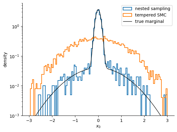

Nested sampling piles onto the narrow spike at the origin, tracking the true marginal; tempered SMC stays spread across the broad background — precisely the mass it undercounts in $\log Z$. The compression curves show why.

Exploring the robustness of Nested Sampling¶

We can probe how differently the two algorithms see the problem using the full particle history. We plot the mean log-likelihood of the population as each method iterates — nested sampling (left) as it compresses, tempered SMC (right) as it heats — on a shared $y$-axis, with a dotted reference at the spike’s typical set, the log-likelihood a sampler must reach to have resolved the spike.

Source

logL = np.sort(np.array(nss_mix.particles.loglikelihood))

# NS live-set mean log-likelihood at each iteration: a window of n_live sorted points,
# stepped by n_delete. Reconstructed from the finalised points — no extra bookkeeping.
starts = np.arange((logL.size - n_live) // n_delete) * n_delete
ns_meanL = np.array([logL[s : s + n_live].mean() for s in starts])
ns_iter = starts / n_live       # equivalent NS iterations (whole-population moves)
smc_meanL = np.array(smc_meanL)

# the spike Gaussian's typical set sits D/2 nats below its peak log-height
spike_ts = float(np.log(np.array(heights[1]))) - D / 2

fig, (ax1, ax2) = plt.subplots(1, 2, figsize=(11, 4), sharey=True)

ax1.plot(ns_iter, ns_meanL, lw=1.4, color="C0", label=r"mean $\log\mathcal{L}$")
ax1.axhline(spike_ts, ls=":", color="k", lw=1.2, label="spike typical set")
ax1.set_ylim(-45, 27)
ax1.set_xlabel("equivalent NS iteration (logL step)")
ax1.set_ylabel(r"$\log \mathcal{L}$")
ax1.set_title("Nested Sampling Compression")
ax1.legend(fontsize=8, loc="lower right")

ax2.plot(np.arange(1, smc_meanL.size + 1), smc_meanL, "o-", ms=3, lw=1.4, color="C1",
         label=r"mean $\log\mathcal{L}$")
ax2.axhline(spike_ts, ls=":", color="k", lw=1.2, label="spike typical set")
ax2.set_xlabel(r"SMC iteration ($\beta$ step)")
ax2.set_title("Tempered SMC Compression")
ax2.legend(fontsize=8, loc="lower right")
fig.tight_layout()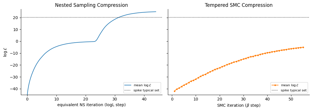

Nested sampling takes uniform steps in the enclosed prior volume, so around the transition — the plateau where the two phases meet — its steps in log-likelihood automatically shorten. Because the volume compression continues uniformly regardless, the effective log-likelihood step readapts to the narrow Gaussian spike and keeps progressing with well-chosen step sizes. Tempered SMC never does: its ensemble climbs off the prior, then plateaus in the background far below the spike, because raising $\beta$ exerts no pull toward a peak that holds almost no probability until $\beta = 1$ — by which point its proposal is far too coarse to find it. Even an extremely fine, fixed $\beta$ schedule stays pathological for the tempering approach.

This is why we set the termination target so deep: across the gap the live points genuinely hold almost nothing, so the usual dlogz = -3 would quit early — hence dlogz = -10. For standard probabilistic problems -3 is a sensible general-purpose default, but this athermal compression is a defining feature of nested sampling, and on many physical systems the deeper compression is worth paying for.

SMC, by contrast, is left at -13.8 even with its fine annealing schedule (target_ess = 0.99, ~55 temperatures). First-order phase transitions are the textbook failure of thermal methods, and precisely the regime nested sampling is built for; this target just makes it explicit.

Synthesis¶

We have demonstrated the nested sampling algorithm and positioned it alongside the SMC approaches already in BlackJAX. On the two problems studied we saw:

• Multimodality (both agree). When the obstacle is an energy barrier between well-resolved modes, both methods draw particles into every well straight from the prior, so tempering and volume compression weight the modes alike and return the same $\log Z$. On the bimodal target the two are interchangeable.

• A phase transition (nested sampling stays robust). When 90% of the evidence hides in a sharp, low-volume spike, the target is a first-order phase transition: nudge $\beta$ past the transition and SMC’s random walk must leap straight from the broad background into the spike, so it never resolves it and its $\log Z$ comes out nats too low. Nested sampling parametrises the path by prior volume instead and keeps compressing straight through the trough — the robustness a volume parametrisation buys at a first-order transition.

Built from primitives. Both samplers are assembled from the same two BlackJAX pieces — a generic outer loop that replaces the worst live points under a rising likelihood constraint, and a pluggable inner kernel that draws the replacements. blackjax.nss fills that slot with a hit-and-run slice sampler; an axis-aligned slice-within-Gibbs move gives blackjax.nsswig instead, and any sampler that can draw from the constrained prior would serve. That modularity is the skeleton shared with SMC, and what lets the preamble’s inner-kernel tuning drop into both.

In practice. Despite these attractive properties, some of nested sampling’s strengths are limited by the difficulty of constrained sampling. The most natural inner kernel is the slice family — a powerful engine, but one that cannot on its own reach the dimensionality that gradient-based HMC does. BlackJAX’s structure-aware design lets one build a Metropolis-within-Gibbs kernel to scale further Yallup, 2026, or bring in Laplace marginalisation of latent variables.

The blackjax.ns package also exposes a generic blackjax.ns.from_mcmc utility for building custom kernels, along with base and adaptive abstractions for further research into practical constrained samplers.