This notebook demonstrates BlackJAX’s two multivariate slice samplers —
blackjax.coordinate_slice and blackjax.slice_sampling — and shows how the
right choice between them is dictated by the geometry of the target.
Core idea. Both samplers are built on the same univariate slice spine Neal, 2003, but they extend it to many dimensions in opposite ways:
coordinate_slice : slice-within-Gibbs -- update each axis's full conditional
                   x_i <- univariate slice on  p(x_i | x_{-i})

slice_sampling   : hit-and-run        -- slice along a single direction
                   d <- direction_proposal(scale);  x <- univariate slice along d
Which one to reach for is a question about geometry, and the answer flips between two classic targets: when the local scale changes with position (a curved target) the per-axis sweep wins; when one global metric is right everywhere (a linear correlation) a preconditioned direction wins.
| target | geometry | winner | why |
|---|---|---|---|
| Neal’s funnel | curved, scale varies with position | coordinate | per-axis adaptive bracketing tracks the local scale gradient-free (NUTS’s one step size misses the neck) |
| tight correlation | a fixed tilted ridge (linear) | hit-and-run | one direction crosses the ridge — if the direction is preconditioned by the covariance |
This notebook demonstrates:
Neal’s Funnel (Curved Geometry) — coordinate slice tracks the position-dependent scale gradient-free, where NUTS’s single tuned step size misses the neck.
A Tight Correlation (Linear Geometry) — a Pathfinder-preconditioned hit-and-run crosses the ridge in one slice, where coordinate/Gibbs crawls.
The Interval Procedure —
doublingvsstepping_out, and how the right choice depends on how well the initialwidthmatches the scale.
import jax
import jax.numpy as jnp
import jax.scipy.stats as jss
import numpy as np
import matplotlib.pyplot as plt

import blackjax
from blackjax.mcmc.slice import direction_proposal, doubling, stepping_out

# Reproducibility
key = jax.random.key(42)

plt.rcParams.update({"figure.dpi": 120, "font.size": 11})


# Generic vmapped runner: coordinate_slice, slice_sampling and nuts all share the
# init / step interface, so only the kernel changes.
def run_chains(algo, rng_key, x0s, n_steps):
    """Run one chain per row of x0s (vmapped); return (n_chains, n_steps, dim)."""

    def chain(k, x0):
        state = algo.init(x0)

        def one(s, kk):
            s, _ = algo.step(kk, s)
            return s, s.position

        _, positions = jax.lax.scan(one, state, jax.random.split(k, n_steps))
        return positions

    return jax.vmap(chain)(jax.random.split(rng_key, x0s.shape[0]), x0s)


def pool(positions):
    """Discard the first half of each chain as burn-in, then pool the rest."""
    n_steps = positions.shape[1]
    return positions[:, n_steps // 2 :, :].reshape(-1, positions.shape[-1])
Section 1: Neal’s Funnel (Curved Geometry)
Neal’s funnel in dimensions has a global scale and coordinates whose spread is set by :
(Following Neal, is parameterized by standard deviation , so has variance 9.)
The neck (small ) is narrow and the mouth (large ) is wide, so the right step size changes with position — a non-linear, curved geometry. The marginal is exactly , which we use as ground truth: a sampler that can’t reach the neck shows up as a too-light left tail.
D = 10  # z dimensions; the funnel lives in D + 1 dims (theta, z[0..D-1])


def funnel_logdensity(x):
    """Neal's funnel: theta ~ N(0, 3),  z_i | theta ~ N(0, exp(theta/2))."""
    theta, z = x[0], x[1:]
    return jss.norm.logpdf(theta, 0.0, 3.0) + jss.norm.logpdf(
        z, 0.0, jnp.exp(theta / 2.0)
    ).sum()


def funnel_truth(rng_key, n):
    """Exact i.i.d. draws from the funnel (the ground truth)."""
    kt, kz = jax.random.split(rng_key)
    theta = jax.random.normal(kt, (n,)) * 3.0
    z = jax.random.normal(kz, (n, D)) * jnp.exp(theta / 2.0)[:, None]
    return jnp.concatenate([theta[:, None], z], axis=1)
Each chain starts from a standard normal draw over the D + 1 coordinates
(theta, z), and we discard the first half as burn-in — so the neck
(theta < -4) and the wide mouth are left for each sampler to reach on its own.
n_chains, n_steps = 64, 1500
key, init_key = jax.random.split(key)
x0s = jax.random.normal(init_key, (n_chains, D + 1))
Coordinate Slice vs Hit-and-Run vs NUTS
Coordinate slice and isotropic hit-and-run are the two slice options; NUTS is the gradient-based reference, warmed up with window adaptation.
key, sk = jax.random.split(key)
coord_funnel = pool(run_chains(blackjax.coordinate_slice(funnel_logdensity), sk, x0s, n_steps))

key, sk = jax.random.split(key)
hr_funnel = pool(run_chains(blackjax.slice_sampling(funnel_logdensity), sk, x0s, n_steps))
key, wk = jax.random.split(key)
warmup = blackjax.window_adaptation(
blackjax.nuts, funnel_logdensity
)
(_, nuts_params), _ = warmup.run(wk, jnp.zeros(D + 1), num_steps=1000)
key, sk = jax.random.split(key)
nuts_funnel = pool(run_chains(blackjax.nuts(funnel_logdensity, **nuts_params), sk, x0s, n_steps))The theta Marginal vs Truth
Truth is . Watch the left tail (the neck): coordinate slice fills it, isotropic hit-and-run does not.
key, gk = jax.random.split(key)
truth = funnel_truth(gk, 50000)


def frac_neck(s):
    return float((np.asarray(s)[:, 0] < -4).mean())


print(f"frac(theta < -4)   truth = {frac_neck(truth):.3f}")
for name, s in [("coordinate_slice", coord_funnel), ("hit-and-run (iso)", hr_funnel), ("NUTS", nuts_funnel)]:
    t = np.asarray(s)[:, 0]
    print(f"  {name:20s} mean={t.mean():+.2f}  frac<-4={frac_neck(s):.3f}")
frac(theta < -4) truth = 0.092
coordinate_slice mean=+0.05 frac<-4=0.077
hit-and-run (iso) mean=-0.29 frac<-4=0.033
NUTS mean=+1.26 frac<-4=0.000
Source
bins = np.linspace(-9.0, 9.0, 61)
fig, ax = plt.subplots(figsize=(8, 5))
ax.hist(np.asarray(truth)[:, 0], bins=bins, density=True, color="0.85", label="truth  N(0,3)")
for name, s in [
    ("coordinate_slice", coord_funnel),
    ("hit-and-run (isotropic)", hr_funnel),
    ("NUTS", nuts_funnel),
]:
    ax.hist(np.asarray(s)[:, 0], bins=bins, density=True, histtype="step", lw=1.8, label=name)
ax.set_xlabel("theta")
ax.set_ylabel("density")
ax.legend()
plt.show()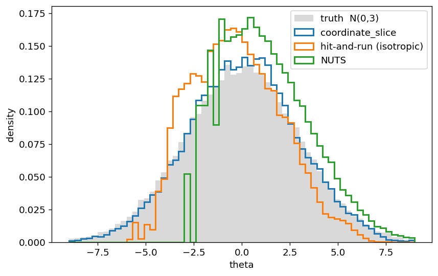
Why coordinate wins here. The funnel is curved: the right scale for is , which changes with position. Coordinate slice updates from its full 1-D conditional and each from its conditional given , and the univariate slice auto-brackets to whatever width that conditional has — tight in the neck, wide in the mouth. It recovers the marginal essentially exactly, and it reaches the neck where gradient-based NUTS’s single tuned step size completely fails to (the classic funnel pathology, usually cured by reparameterization), all without gradients or step-size tuning. Isotropic hit-and-run can’t follow the curve: a straight direction that lowers drags the ’s outside the shrinking shell, so the chain can’t descend into the neck and its left tail stays too light. This is exactly Neal’s funnel verdict — the single-variable sweep is the winner.
Section 2: A Tight Correlation (Linear Geometry)
Now flip the geometry: a zero-mean 2-D Gaussian with . Its mass is a thin tilted ridge along . Here the right metric is the same everywhere (it’s linear) — the case hit-and-run was made for, provided its directions are preconditioned by that metric.
rho = 0.98
Sigma = jnp.array([[1.0, rho], [rho, 1.0]])


def corr_logdensity(x):
    return jss.multivariate_normal.logpdf(x, jnp.zeros(2), Sigma)


def run_one(algo, rng_key, n, x0):
    """A single chain from x0; return its positions."""
    state = algo.init(x0)

    def one(s, k):
        s, _ = algo.step(k, s)
        return s, s.position

    _, pos = jax.lax.scan(one, state, jax.random.split(rng_key, n))
    return pos


def ess_slow(samples):
    """Crude ESS along the slow ridge axis (1,1)/sqrt2 via summed autocorr."""
    u = jnp.array([1.0, 1.0]) / jnp.sqrt(2.0)
    x = jnp.asarray(samples) @ u
    x = x - x.mean()
    n = x.shape[0]
    var = jnp.mean(x * x)
    acf = jnp.array([jnp.mean(x[: n - k] * x[k:]) / var for k in range(1, n // 3)])
    neg = int(jnp.argmax(acf < 0))  # Geyer initial-positive cut
    tau = 1.0 + 2.0 * float(jnp.sum(acf[:neg]))
    return n / tau


N = 6000
burnin = N // 2
x0_corr = jnp.array([3.0, 3.0])  # off-mode: ~3 sigma out along the ridge
Fitting the Covariance with Pathfinder
In practice you don’t have Sigma. A cheap way to get it is Pathfinder
(blackjax.pathfinder) Zhang et al., 2022, an L-BFGS variational
pre-run that returns a Gaussian approximation; its covariance is what we feed to
direction_proposal(scale=cholesky(cov)). This is an example of a pre-tuning step
that works with slice sampling, similar to the window_adaptation used earlier to
pre-tune NUTS. We use a single Pathfinder run for minimal pretuning, but
multi-path Pathfinder is the more robust standard choice in practice.
def pathfinder_cov(rng_key, logdensity_fn, dim, radius=3.0):
    """Single-run Pathfinder; return the covariance of its Gaussian fit."""
    ka, kb, kc = jax.random.split(rng_key, 3)
    start = jax.random.normal(ka, (dim,)) * radius
    state, _ = blackjax.pathfinder.approximate(kb, logdensity_fn, start)
    draws, _ = blackjax.pathfinder.sample(kc, state, 6000)
    return jnp.cov(jnp.asarray(draws).T)


key, pk = jax.random.split(key)
cov_fit = pathfinder_cov(pk, corr_logdensity, 2)
L_fit = jnp.linalg.cholesky(cov_fit)
corr_fit = float(cov_fit[0, 1] / jnp.sqrt(cov_fit[0, 0] * cov_fit[1, 1]))
print(f"Pathfinder-fitted correlation = {corr_fit:+.3f}   (true rho = {rho})")
Pathfinder-fitted correlation = +0.981 (true rho = 0.98)
Three Samplers on the Ridge
coordinate_slice— axis-aligned; each conditional has variance , so it inches across the ridge (Gibbs on a correlated Gaussian).hit-and-run, uninformed — isotropic directions; most miss the ridge direction, so jumps along it are small.
hit-and-run, Pathfinder-fitted —
direction_proposal(scale=L_fit)aims the directions along the ridge, so one slice traverses it.
All three start off-mode, ~3σ out along the ridge at (3, 3), so the plotted
paths show convergence (how fast each reaches the bulk) as well as stationary
mixing. ESS is measured after discarding the first half as burn-in, so it still
reflects stationary mixing, not the transient.
key, k1 = jax.random.split(key)
coord_corr = run_one(blackjax.coordinate_slice(corr_logdensity), k1, N, x0_corr)

key, k2 = jax.random.split(key)
hr_iso_corr = run_one(blackjax.slice_sampling(corr_logdensity), k2, N, x0_corr)

key, k3 = jax.random.split(key)
hr_fit_corr = run_one(
    blackjax.slice_sampling(corr_logdensity, proposal_generator=direction_proposal(scale=L_fit)),
    k3,
    N,
    x0_corr,
)

runs = [
    ("coordinate_slice", coord_corr),
    ("hit-and-run (uninformed)", hr_iso_corr),
    ("hit-and-run (Pathfinder)", hr_fit_corr),
]
print(f"slow-axis ESS (of {N - burnin} post-burn-in), start = {tuple(float(v) for v in x0_corr)}:")
for name, s in runs:
    print(f"  {name:28s} {ess_slow(s[burnin:]):7.1f}")
slow-axis ESS (of 3000 post-burn-in), start = (3.0, 3.0):
coordinate_slice 56.8
hit-and-run (uninformed) 124.3
hit-and-run (Pathfinder) 1087.2
Source
# truth contours: k * cholesky(Sigma) @ unit_circle for k = 1, 2
phi = np.linspace(0.0, 2.0 * np.pi, 200)
circle = np.stack([np.cos(phi), np.sin(phi)])
L_true = np.asarray(jnp.linalg.cholesky(Sigma))

fig, axes = plt.subplots(1, 3, figsize=(13.5, 4.6), sharex=True, sharey=True)
for ax, (name, s) in zip(axes, runs):
    s = np.asarray(s)
    # first 400 steps show the off-mode approach
    ax.plot(s[:400, 0], s[:400, 1], "-o", ms=2.5, lw=0.4, alpha=0.5)
    for k in (1, 2):
        e = k * L_true @ circle
        ax.plot(e[0], e[1], "k--", lw=1.1)
    ax.set_title(f"{name}\nslow-axis ESS = {ess_slow(s[burnin:]):.0f} / {N - burnin}", fontsize=10)
    ax.set_xlabel("x[0]")
    ax.set_aspect("equal")
axes[0].set_ylabel("x[1]")
fig.tight_layout()
plt.show()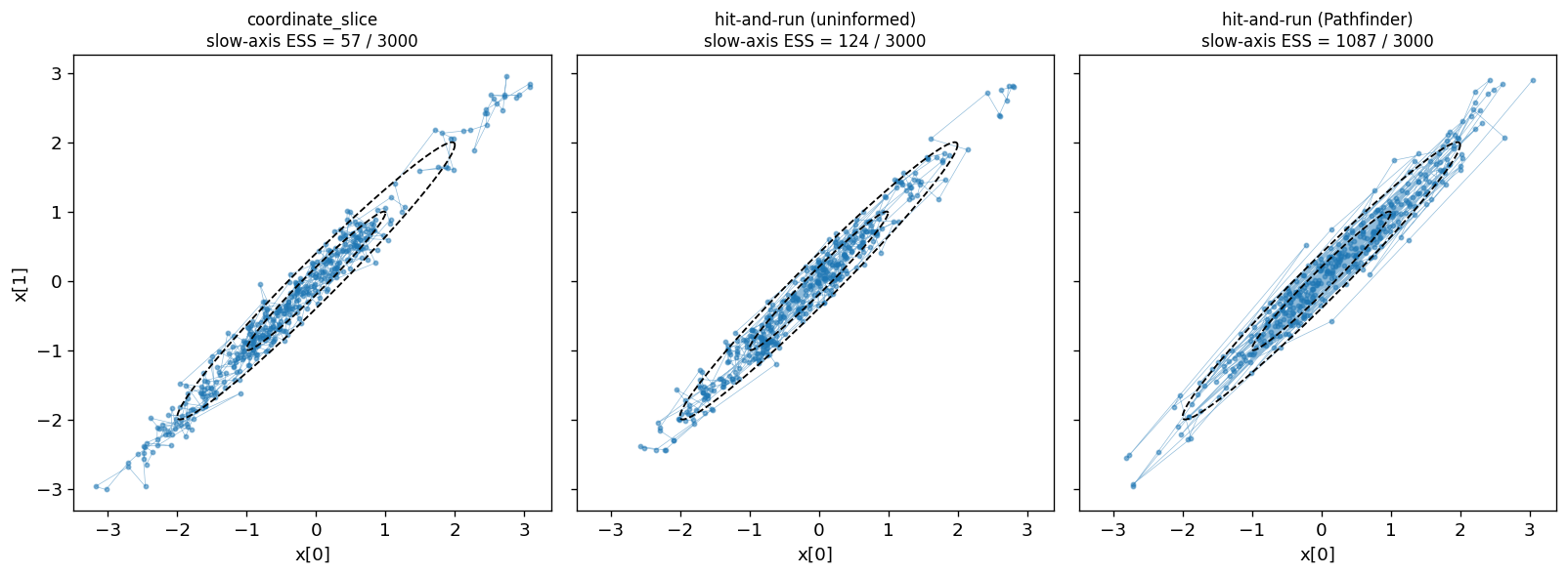
Trace of the Diagonal Coordinate
The ESS gap is clearest along the slow ridge axis : both coordinate slice and isotropic hit-and-run mix slowly along this tightly correlated direction, while the Pathfinder-fitted hit-and-run decorrelates quickly.
Source
u_slow = np.array([1.0, 1.0]) / np.sqrt(2.0)

fig, axes = plt.subplots(3, 1, figsize=(10, 7), sharex=True, sharey=True)
for ax, (name, s) in zip(axes, runs):
    proj = np.asarray(s) @ u_slow
    ax.plot(proj, lw=0.5)
    ax.axhline(0.0, color="k", lw=0.6, alpha=0.6)        # target mean
    ax.axvline(burnin, color="0.6", ls=":", lw=1.2)      # end of burn-in
    ax.set_ylabel("diag. coord")
    ax.set_title(
        f"{name}   slow-axis ESS = {ess_slow(s[burnin:]):.0f} / {N - burnin}",
        fontsize=9, loc="left",
    )
axes[-1].set_xlabel("iteration")
fig.tight_layout()
plt.show()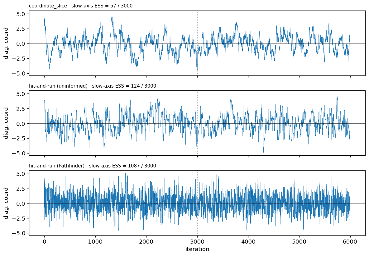
Section 3: The Interval Procedure — Doubling vs Stepping-Out
Every univariate slice first finds a bracket around the slice, then
shrinks to draw the new point. The bracket step is pluggable — one keyword on
either sampler (interval=doubling, the default, or interval=stepping_out):
stepping_out(Neal Fig. 3) grows the bracket linearly from the initialwidth, splitting a step budget (max_expansions) across the two sides.doubling(Neal Fig. 4) grows it geometrically — doubling one random side per step — plus a Fig. 6 acceptance test to stay reversible.
Two cost diagnostics ride on SliceInfo (shown per step below):
num_expansions (bracket-growth steps, capped by max_expansions) and
num_shrink (candidate draws in the shrink phase, capped by max_shrinkage).
The choice comes down to how well the initial width matches the scale — the
very scale Pathfinder fit for us in Section 2:
Know the scale (
width≈ the slice width) → stepping-out is most efficient: it brackets in a step or two, with no acceptance-test overhead.Get it badly wrong (
widthfar too small) → doubling wins: geometric growth reaches the slice inlog2steps where linear stepping-out crawls.
def reach_logdensity(x):
    return jss.norm.logpdf(x[0], 0.0, 10.0)  # wide 1-D target; the slice spans ~ +-25


def ess_1d(x):
    x = jnp.asarray(x) - jnp.mean(x)
    n = x.shape[0]
    var = jnp.mean(x * x)
    acf = jnp.array([jnp.mean(x[: n - k] * x[k:]) / var for k in range(1, n // 3)])
    neg = int(jnp.argmax(acf < 0))
    return float(n / (1.0 + 2.0 * float(jnp.sum(acf[:neg]))))


def interval_run(algo, rng_key, n):
    state = algo.init(jnp.array([0.0]))

    def one(s, k):
        s, info = algo.step(k, s)
        return s, (s.position[0], info.num_expansions, info.num_shrink)

    _, out = jax.lax.scan(one, state, jax.random.split(rng_key, n))
    return out


M = 6000
print("1-D N(0, 10), max_expansions = 60   (truth std = 10)")
print(f"{'width':>6s} {'interval':13s} {'std':>5s} {'exp/step':>9s} "
      f"{'shrink/step':>12s} {'ESS':>6s} {'evals/eff':>10s}")
for width, tag in [(20.0, "width tuned to the scale"), (0.5, "width 40x too small")]:
    for name, interval in [("doubling", doubling), ("stepping_out", stepping_out)]:
        key, sk = jax.random.split(key)
        algo = blackjax.slice_sampling(
            reach_logdensity, width=width, interval=interval, max_expansions=60
        )
        pos, nexp, nshr = interval_run(algo, sk, M)
        h = slice(M // 2, None)
        e, s = float(nexp[h].mean()), float(nshr[h].mean())
        ess = ess_1d(pos[h])
        print(f"{width:6.1f} {name:13s} {float(jnp.std(pos[h])):5.1f} {e:9.1f} {s:12.1f} "
              f"{ess:6.0f} {(e + s) * (M // 2) / ess:10.1f}")
    print(f"       -> {tag}\n")
1-D N(0, 10), max_expansions = 60 (truth std = 10)
width interval std exp/step shrink/step ESS evals/eff
20.0 doubling 10.0 2.5 2.9 2997 5.4
  20.0 stepping_out   10.2       1.6          1.6   2973        3.2
       -> width tuned to the scale
0.5 doubling 10.1 7.8 2.9 3000 10.7
   0.5 stepping_out   10.1      38.1          1.0    550      213.3
       -> width 40x too small
Reading the results. Both widths recover the target (std ≈ 10) — the swap
never breaks correctness — but efficiency flips. With the width tuned to the
scale, stepping_out is the cheapest (it brackets in ~1–2 steps and skips
doubling’s acceptance test). With the width badly wrong, doubling is far
cheaper: it reaches the slice while stepping-out crawls out linearly and its ESS
collapses. So if a fit like Pathfinder hands you the scale, prefer stepping_out;
otherwise keep the robust doubling default.
Synthesis
The two halves are mirror images, and the deciding factor is whether the target’s local metric is constant:
Funnel (curved). No single metric is right everywhere, so a fixed-direction hit-and-run — even with a covariance — can’t win. What works is matching the conditional structure: coordinate slice’s per-axis adaptive bracketing, which here outdoes gradient-based NUTS — whose one tuned step size can’t resolve the neck — without gradients or tuning. (Neal’s own conclusion.)
Correlation (linear). One global metric is right everywhere, so coordinate/Gibbs crawls while a preconditioned hit-and-run crosses the ridge in a single slice. You don’t need the oracle
Sigma: a cheap Pathfinder fit recovers it, and thescale=argument ofdirection_proposalis the seam that consumes it. The same seam is what nested slice sampling rides — it preconditions the hit-and-run direction with the running live-point covariance, Pathfinder’s fitted metric re-estimated as the constrained prior contracts.
Quick-reference: which slice sampler to use.
| Situation | Reach for | Why |
|---|---|---|
| Curved / axis-structured target (scale varies with position) | coordinate_slice | per-axis adaptive bracketing, tuning-free, gradient-free |
| (Locally) linear correlation | slice_sampling + direction_proposal(scale=L) | one preconditioned slice crosses the ridge |
| You have a covariance fit (e.g. Pathfinder) | slice_sampling(..., interval=stepping_out) | width matches the scale → brackets in 1–2 steps |
width / scale poorly known | slice_sampling(..., interval=doubling) (default) | geometric growth reaches the slice in log2 steps |
In practice. As a black-box default, coordinate slice is the most robust of the three — tuning-free, gradient-free, and unbothered by curved, axis-structured geometry. To go beyond a black-box sampler, combining the two ideas is a good idea: block the variables and run a multivariate slice (hit-and-run) within a Gibbs sweep, so each block gets a direction preconditioned to its own local correlation.
- Neal, R. M. (2003). Slice sampling. The Annals of Statistics, 31(3), 705–767. 10.1214/aos/1056562461
- Zhang, L., Carpenter, B., Gelman, A., & Vehtari, A. (2022). Pathfinder: Parallel quasi-Newton variational inference.