How to use Laplace-preconditioned HMC

How to use Laplace-preconditioned HMC#

Hierarchical models often have the form:

phi   ~ p(phi)               # hyperparameters (low-dimensional)
theta ~ p(theta | phi)       # latent variables (potentially large)
y     ~ p(y | theta, phi)    # observations

The joint posterior p(theta, phi | y) can be geometrically difficult to sample directly: phi and theta are strongly correlated and theta is often high-dimensional. Laplace HMC sidesteps this by marginalising out theta analytically (via the Laplace approximation) and running HMC only on the low-dimensional phi.

The key idea: at each leapfrog step, an L-BFGS solver finds theta*(phi) = argmax_theta log p(theta, phi, y), and the Laplace-approximate marginal log p̂(phi | y) is used as the HMC potential. Gradients w.r.t. phi are computed via the implicit function theorem — the optimisation iterations are not unrolled.

When to use it

The conditional p(theta | phi, y) is unimodal and roughly Gaussian (the approximation is exact for Gaussian-Gaussian models).
dim(phi) is small and dim(theta) is large; you want to sample only phi.
You need posterior samples of theta — these can be drawn cheaply from the Laplace-approximate conditional after sampling phi.

from datetime import date

import jax
import jax.numpy as jnp
import jax.scipy.stats as stats
import matplotlib.pyplot as plt
import numpy as np

import blackjax
from blackjax.mcmc.laplace_marginal import laplace_marginal_factory
from blackjax.util import run_inference_algorithm

rng_key = jax.random.key(int(date.today().strftime("%Y%m%d")))

The model#

We use a conjugate Gaussian hierarchy where the Laplace approximation is exact, so we can verify the sampler against the true marginal:

log_sigma  ~ N(0, 3²)                    # log hyperparameter (phi), scalar
theta      ~ N(0, exp(log_sigma)² · I_n) # latent vector, n-dimensional
y          ~ N(theta, I_n)               # observations

The exact marginal is y_i ~ N(0, sigma² + 1) independently.

n = 20  # latent dimension

# Generate data
true_log_sigma = jnp.log(jnp.array(2.0))
rng_key, data_key = jax.random.split(rng_key)
true_theta = jax.random.normal(data_key, (n,)) * jnp.exp(true_log_sigma)
rng_key, obs_key = jax.random.split(rng_key)
y_obs = true_theta + jax.random.normal(obs_key, (n,))


def log_joint(theta, log_sigma):
    """log p(theta, log_sigma, y).  theta is the latent, log_sigma is phi."""
    sigma = jnp.exp(log_sigma)
    log_prior_phi = stats.norm.logpdf(log_sigma, 0.0, 3.0)
    log_prior_theta = stats.norm.logpdf(theta, 0.0, sigma).sum()
    log_lik = stats.norm.logpdf(y_obs, theta, 1.0).sum()
    return log_prior_phi + log_prior_theta + log_lik


def exact_log_marginal(log_sigma):
    """Closed-form marginal p̂(log_sigma | y) for verification."""
    sigma = jnp.exp(log_sigma)
    log_prior_phi = stats.norm.logpdf(log_sigma, 0.0, 3.0)
    var_marg = sigma**2 + 1.0
    log_lik_marg = stats.norm.logpdf(y_obs, 0.0, jnp.sqrt(var_marg)).sum()
    return log_prior_phi + log_lik_marg

Running `blackjax.laplace_hmc`#

The only change from standard blackjax.hmc is:

Pass log_joint(theta, phi) instead of a log-density over all variables.
Pass theta_init to fix the latent dimension and provide a cold-start hint for the L-BFGS solver.

theta_init = jnp.zeros(n)
phi_init = jnp.array(0.0)

sampler = blackjax.laplace_hmc(
    log_joint,
    theta_init=theta_init,
    step_size=0.3,
    inverse_mass_matrix=jnp.ones(1),
    num_integration_steps=10,
    maxiter=100,  # L-BFGS iterations per leapfrog step
)

rng_key, run_key = jax.random.split(rng_key)
final_state, (states, infos) = run_inference_algorithm(
    run_key,
    sampler,
    num_steps=1_000,
    initial_position=phi_init,
    transform=lambda state, info: (state, info),
)

phi_samples = states.position          # shape (1000,)
theta_star_samples = states.theta_star # shape (1000, n) — MAP theta at each phi

print(f"Acceptance rate:  {infos.acceptance_rate.mean():.2f}")
print(f"Divergences:      {infos.is_divergent.sum()}")
print(f"phi posterior mean:  {phi_samples.mean():.3f}  (true log_sigma={true_log_sigma:.3f})")

Acceptance rate:  0.74
Divergences:      0
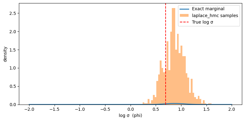
phi posterior mean:  0.733  (true log_sigma=0.693)

Verify against the exact marginal#

Since our model is Gaussian, we can compare the sampled phi distribution against the true marginal log-density:

../_images/7c89fbe51b0ea18b5e8c2f38f12d463b32979da00a42c48f08b67c76e21badb1.png

Sampling theta given phi#

states.theta_star contains the MAP estimate of theta at each accepted phi, not a posterior sample. To draw proper posterior samples of theta, use laplace.sample_theta:

laplace = laplace_marginal_factory(log_joint, theta_init, maxiter=100)

rng_key, *theta_keys = jax.random.split(rng_key, len(phi_samples) + 1)
theta_keys = jnp.array(theta_keys)

# Draw one theta sample per phi sample
theta_samples = jax.vmap(laplace.sample_theta)(
    jnp.array(theta_keys), phi_samples, theta_star_samples
)  # shape (1000, n)

print(f"theta posterior mean (first 5): {theta_samples[:, :5].mean(axis=0)}")

theta posterior mean (first 5): [ 1.78022    -0.16777255 -2.0537927   3.331983    2.5445073 ]

Using `laplace_mhmc` for better ESS#

blackjax.laplace_mhmc uses a multinomial trajectory proposal instead of the standard endpoint + Metropolis–Hastings accept/reject step. This typically gives higher ESS per leapfrog gradient evaluation at the cost of always accepting (no rejection):

sampler_mhmc = blackjax.laplace_mhmc(
    log_joint,
    theta_init=theta_init,
    step_size=0.3,
    inverse_mass_matrix=jnp.ones(1),
    num_integration_steps=10,
    maxiter=100,
)

rng_key, run_key = jax.random.split(rng_key)
_, (states_mhmc, _) = run_inference_algorithm(
    run_key,
    sampler_mhmc,
    num_steps=1_000,
    initial_position=phi_init,
    transform=lambda state, info: (state, info),
)

ess_hmc  = blackjax.ess(phi_samples[None])
ess_mhmc = blackjax.ess(states_mhmc.position[None])
print(f"ESS laplace_hmc:  {ess_hmc:.1f}")
print(f"ESS laplace_mhmc: {ess_mhmc:.1f}")

ESS laplace_hmc:  849.1
ESS laplace_mhmc: 952.6

Practical notes#

Choosing maxiter The L-BFGS solver runs maxiter iterations at every leapfrog step. The warm-starting from theta_star means only a few iterations are typically needed once the chain is mixing. Start with maxiter=30 (the default) and increase if you see NaN log-densities or divergences.

Checking the approximation quality The Laplace approximation is accurate when p(theta | phi, y) is well-concentrated and unimodal. Red flags: high divergence counts, bimodal theta_star distributions, or rhat > 1.01 on phi samples despite seemingly good acceptance rates.

Dimension constraints The Hessian computation is O(dim(theta)²) memory and O(dim(theta)³) per step. Practical upper bound is dim(theta) ~ 500–1000 on a single device. For larger latent spaces, consider sparse or structured approximations, or switching to joint sampling with blackjax.nuts + better geometry.

Dynamic variant blackjax.laplace_dhmc and blackjax.laplace_dmhmc use dynamic trajectory length (NUTS-style), removing the need to hand-tune num_integration_steps. The interface is identical; just swap the sampler name.