Use with Funsor

Funsor is a library of functional tensors for probabilistic programming. It generalises the tensor interface by treating arrays as functions over named variables rather than positionally indexed grids. The central consequence for MCMC: Funsor can exactly marginalise discrete latent variables via variable elimination, turning a sum over K discrete states into a fused JAX operation that is fully compatible with jax.jit and jax.grad.

This makes Funsor the natural complement to BlackJax for models that mix discrete and continuous latent variables — Gaussian Mixture Models, Hidden Markov Models, mixed-membership models — where gradient-based samplers such as NUTS would otherwise be inapplicable because discrete variables block automatic differentiation.

In this notebook we fit a Gaussian Mixture Model with K=3 components. The discrete component assignments z_i are marginalised analytically by Funsor; BlackJax NUTS then samples the continuous parameters μ and π.

Before you start

You will need Funsor to run this example:

pip install "funsor>=0.4.7"

Setup and data

import jax
import jax.numpy as jnp
import numpy as np
import blackjax

import funsor
import funsor.ops as ops

funsor.set_backend("jax")          # must be called before Tensor/Variable are used

from funsor.domains import Bint
from funsor.tensor import Tensor
from funsor.terms import Variable
from funsor.jax.distributions import Categorical, Normal

from datetime import date
rng_key = jax.random.key(int(date.today().strftime("%Y%m%d")))

We generate synthetic data from a three-component Gaussian mixture so we can verify that the sampler recovers the true parameters.

Show code cell content

Hide code cell content

K, N = 3, 300
true_mu = np.array([-4.0, 0.0, 4.0])
true_pi = np.array([0.3,  0.4, 0.3])

rng    = np.random.default_rng(42)
z_true = rng.choice(K, size=N, p=true_pi)
data   = jnp.array(rng.normal(true_mu[z_true], 1.0), dtype=jnp.float32)

print(f"N={N} observations, K={K} components")
print(f"True means : {true_mu}")
print(f"True weights: {true_pi}")

N=300 observations, K=3 components
True means : [-4.  0.  4.]
True weights: [0.3 0.4 0.3]

The model and log-density

The generative model is:

π   ~ Dirichlet(1, 1, 1)        # mixing weights  (continuous)
μ_k ~ Normal(0, 5)              # component means (continuous)
z_i ~ Categorical(π)            # assignment      (discrete — marginalised)
x_i | z_i ~ Normal(μ[z_i], 1)  # likelihood

Because z_i is discrete, direct gradient-based inference is impossible. Funsor solves this by treating the sum over assignments as a symbolic computation graph that JAX can differentiate through. Three Funsor primitives do all the work:

• Tensor(arr, {"name": Bint[size]}) — wraps a JAX array so its axis is addressable by name rather than by integer position.

• Variable("z", Bint[K]) — a free (unevaluated) discrete variable ranging over {0, …, K-1}.

• f(k=z) — substitution: renames the "k" axis to "z", transferring the name so that expressions over different named axes broadcast correctly.

• Normal(loc=..., scale=..., value=x) / Categorical(probs=..., value=z) — distribution objects from funsor.jax.distributions that accept a Funsor as value and return the log-probability as a Funsor over that variable’s named dimensions. Distinct named dimensions in loc and value broadcast as an outer product automatically.

The mixing weights π live on the K-simplex. Rather than sampling all K components of log_pi (which leaves a constant-shift null direction that confuses the mass matrix), we fix the first logit to zero and sample only K−1 free parameters. The map ℝ^{K-1} → Δ^{K-1} is bijective, so no Jacobian correction is needed.

def gmm_logdensity(position):
    mu     = position["mu"]          # (K,)   component means
    log_pi = position["log_pi"]      # (K-1,) unconstrained free logits
    # Prepend a fixed zero so softmax maps K-1 reals bijectively onto Δ^{K-1}.
    pi = jax.nn.softmax(jnp.concatenate([jnp.zeros(1), log_pi]))   # (K,)

    # ── Named Funsor tensors ─────────────────────────────────────────────────
    # Tensor(arr, inputs): arr is indexed by the dimensions named in inputs.
    # pi_f has no named dim: Categorical indexes it internally via value=z.
    mu_f = Tensor(mu,   {"k": Bint[K]})   # mu_f[k]  for k ∈ {0, …, K-1}
    pi_f = Tensor(pi,   {})               # (K,) simplex, no named dim
    x_f  = Tensor(data, {"n": Bint[N]})   # x_f[n]   for n ∈ {0, …, N-1}

    # ── Discrete variable: component assignment ──────────────────────────────
    z = Variable("z", Bint[K])

    # ── log p(z | π) — Categorical, Funsor over {"z"} ───────────────────────
    log_cat_prior = Categorical(probs=pi_f, value=z)              # inputs: {"z": Bint[K]}

    # ── log p(x_n | z) — Normal likelihood, Funsor over {"z", "n"} ──────────
    # mu_f(k=z) substitutes k→z: Funsor over {"z": Bint[K]}.
    # Normal's loc depends on "z" and value depends on "n", so the result
    # spans both dimensions automatically as an outer product.
    mu_z    = mu_f(k=z)
    log_lik = Normal(loc=mu_z, scale=1.0, value=x_f)             # inputs: {"z": Bint[K], "n": Bint[N]}

    # ── Exact marginalisation of z ───────────────────────────────────────────
    # reduce(logaddexp, "z") computes log Σ_z exp(log_joint) for every n.
    # Funsor evaluates all K states and combines with logsumexp inside JAX —
    # the result is fully differentiable w.r.t. mu and pi.
    log_joint      = log_cat_prior + log_lik                      # inputs: {"z": Bint[K], "n": Bint[N]}
    log_marginal_n = log_joint.reduce(ops.logaddexp, "z")         # inputs: {"n": Bint[N]}

    # ── μ prior: μ_k ~ Normal(0, 5), summed over K components ───────────────
    log_mu_prior = Normal(loc=0., scale=5., value=mu_f).reduce(ops.add, "k")

    # ── Total log-density ────────────────────────────────────────────────────
    log_p = log_marginal_n.reduce(ops.add, "n")                   # scalar Funsor, inputs: {}
    return log_p.data + log_mu_prior.data

Let us verify that the log-density is finite at a sensible initialisation and that jax.grad can differentiate through the Funsor marginalisation:

position0 = {
    "mu":     jnp.array([-3., 0., 3.]),
    "log_pi": jnp.zeros(K - 1),   # K-1 free logits; first logit fixed at 0
}
print("log p(data | init):", gmm_logdensity(position0))
print("grad w.r.t. mu    :", jax.grad(gmm_logdensity)(position0)["mu"])

log p(data | init): -813.15216

grad w.r.t. mu    : [-80.09981    4.946947  69.5648  ]

Window adaptation

BlackJax’s window adaptation tunes the NUTS step size and mass matrix during a warmup phase. Here we run 1000 warmup steps, after which the kernel is ready for sampling.

%%time

rng_key, warmup_key = jax.random.split(rng_key)

adapt = blackjax.window_adaptation(blackjax.nuts, gmm_logdensity)
(last_state, parameters), _ = adapt.run(warmup_key, position0, num_steps=1000)
kernel = blackjax.nuts(gmm_logdensity, **parameters).step

CPU times: user 3.54 s, sys: 173 ms, total: 3.71 s
Wall time: 1.67 s

Inference loop

Show code cell content

Hide code cell content

def inference_loop(rng_key, kernel, initial_state, num_samples):
    @jax.jit
    def one_step(state, rng_key):
        state, info = kernel(rng_key, state)
        return state, (state, info)

    keys = jax.random.split(rng_key, num_samples)
    _, (states, infos) = jax.lax.scan(one_step, initial_state, keys)
    return states, infos

%%time

rng_key, sample_key = jax.random.split(rng_key)
states, infos = inference_loop(sample_key, kernel, last_state, num_samples=1000)

CPU times: user 2.55 s, sys: 34.2 ms, total: 2.58 s
Wall time: 1.05 s

Results

Note

GMMs are invariant to permutation of component labels. NUTS converges to one of the K! symmetric modes; the component indices carry no absolute meaning across runs with different random seeds.

import matplotlib.pyplot as plt

mu_samples = states.position["mu"]
# Reconstruct full K-simplex from K-1 free logits.
pi_samples = jax.vmap(
    lambda lp: jax.nn.softmax(jnp.concatenate([jnp.zeros(1), lp]))
)(states.position["log_pi"])

# Resolve label switching: sort components by ascending mean value so the
# plotting order matches true_mu = [-4, 0, 4].
sort_idx   = jnp.argsort(mu_samples, axis=1)
mu_samples = jnp.take_along_axis(mu_samples, sort_idx, axis=1)
pi_samples = jnp.take_along_axis(pi_samples, sort_idx, axis=1)

fig, axes = plt.subplots(2, K, figsize=(9, 4), sharey="row")
for k in range(K):
    axes[0, k].hist(np.array(mu_samples[:, k]), bins=40, density=True)
    axes[0, k].axvline(true_mu[k], color="red", linestyle="--", label="true")
    axes[0, k].set_title(f"μ[{k}]")
    axes[1, k].hist(np.array(pi_samples[:, k]), bins=40, density=True)
    axes[1, k].axvline(true_pi[k], color="red", linestyle="--", label="true")
    axes[1, k].set_title(f"π[{k}]")
axes[0, 0].legend()
plt.tight_layout();

Show code cell source

Hide code cell source

print("Posterior E[μ]:", mu_samples.mean(0).round(2), "  true:", true_mu)
print("Posterior E[π]:", pi_samples.mean(0).round(2), "  true:", true_pi)

accept = float(infos.acceptance_rate.mean())
print(f"Mean acceptance rate: {accept:.2f}")

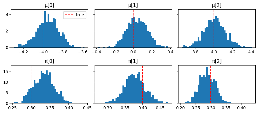
Posterior E[μ]: [-3.9599998  0.05       4.0099998]   true: [-4.  0.  4.]
Posterior E[π]: [0.34 0.38 0.29]   true: [0.3 0.4 0.3]
Mean acceptance rate: 0.90

Alternative: NumPyro model syntax

The pure Funsor approach above requires writing the factor graph explicitly. If you already use NumPyro, you can write the model in the familiar numpyro.sample / numpyro.plate style and let Funsor handle the discrete marginalisation transparently via the @config_enumerate decorator.

Under the hood, initialize_model detects the decorated discrete sites and wires in Funsor’s variable elimination automatically. The continuous parameters are reparameterised (e.g. π via a stick-breaking transform onto the simplex), and the returned potential_fn is fully JAX-differentiable — no changes to the BlackJax call site are required.

Before you start

You will need NumPyro in addition to Funsor:

pip install numpyro "funsor>=0.4.7"

import numpyro
import numpyro.distributions as dist
from numpyro.contrib.funsor import config_enumerate
from numpyro.infer.util import initialize_model

The model is written identically to a standard NumPyro model. The only addition is @config_enumerate, which marks the discrete site z for enumeration. Priors and the likelihood are expressed with NumPyro distributions; no manual log-prob arithmetic is needed.

@config_enumerate
def gmm_model_npy(data, K):
    # Continuous parameters — sampled by BlackJax NUTS
    pi = numpyro.sample("pi", dist.Dirichlet(jnp.ones(K)))
    with numpyro.plate("components", K):
        mu = numpyro.sample("mu", dist.Normal(0.0, 5.0))

    # Discrete assignment — Funsor marginalises this out
    with numpyro.plate("obs", len(data)):
        z = numpyro.sample("z", dist.Categorical(pi))
        numpyro.sample("x", dist.Normal(mu[z], 1.0), obs=data)

initialize_model returns an initial position containing only the continuous variables (in unconstrained space) and a potential_fn_gen that already wraps the Funsor enumeration — the same pattern used in the plain NumPyro tutorial.

rng_key, init_key_npy = jax.random.split(rng_key)

init_params_npy, potential_fn_gen_npy, *_ = initialize_model(
    init_key_npy,
    gmm_model_npy,
    model_args=(data, K),
    dynamic_args=True,
)
initial_position_npy = init_params_npy.z
print("Sites and shapes:", {k: v.shape for k, v in initial_position_npy.items()})

Sites and shapes: {'pi': (2,), 'mu': (3,)}

Note

pi has shape (K-1,) here because NumPyro automatically applies a stick-breaking transform, mapping the (K-1)-dimensional unconstrained space bijectively onto the K-simplex.

logdensity_fn_npy = lambda position: -potential_fn_gen_npy(data, K)(position)

print("log p(data | init):", logdensity_fn_npy(initial_position_npy))
print("grad w.r.t. mu    :", jax.grad(logdensity_fn_npy)(initial_position_npy)["mu"])

log p(data | init): -1674.233
grad w.r.t. mu    : [ -56.92576  262.88333 -291.6114 ]

Window adaptation and the inference loop are identical to before.

%%time

rng_key, warmup_key_npy = jax.random.split(rng_key)

adapt_npy = blackjax.window_adaptation(blackjax.nuts, logdensity_fn_npy)
(last_state_npy, params_npy), _ = adapt_npy.run(
    warmup_key_npy, initial_position_npy, num_steps=1000
)
kernel_npy = blackjax.nuts(logdensity_fn_npy, **params_npy).step

CPU times: user 3.22 s, sys: 90.1 ms, total: 3.31 s
Wall time: 1.42 s

%%time

rng_key, sample_key_npy = jax.random.split(rng_key)
states_npy, infos_npy = inference_loop(
    sample_key_npy, kernel_npy, last_state_npy, num_samples=1000
)

CPU times: user 2.86 s, sys: 33.3 ms, total: 2.89 s
Wall time: 1.17 s

To recover π on the simplex, apply the stick-breaking transform to the unconstrained samples.

from numpyro.distributions.transforms import StickBreakingTransform

mu_samples_npy = states_npy.position["mu"]
pi_samples_npy = jax.vmap(StickBreakingTransform())(states_npy.position["pi"])

sort_idx_npy   = jnp.argsort(mu_samples_npy, axis=1)
mu_samples_npy = jnp.take_along_axis(mu_samples_npy, sort_idx_npy, axis=1)
pi_samples_npy = jnp.take_along_axis(pi_samples_npy, sort_idx_npy, axis=1)

fig, axes = plt.subplots(2, K, figsize=(9, 4), sharey="row")
for k in range(K):
    axes[0, k].hist(np.array(mu_samples_npy[:, k]), bins=40, density=True)
    axes[0, k].axvline(true_mu[k], color="red", linestyle="--", label="true")
    axes[0, k].set_title(f"μ[{k}]")
    axes[1, k].hist(np.array(pi_samples_npy[:, k]), bins=40, density=True)
    axes[1, k].axvline(true_pi[k], color="red", linestyle="--", label="true")
    axes[1, k].set_title(f"π[{k}]")
axes[0, 0].legend()
plt.tight_layout();

Show code cell source

Hide code cell source

print("Posterior E[μ]:", mu_samples_npy.mean(0).round(2), "  true:", true_mu)
print("Posterior E[π]:", pi_samples_npy.mean(0).round(2), "  true:", true_pi)
print(f"Mean acceptance rate: {float(infos_npy.acceptance_rate.mean()):.2f}")

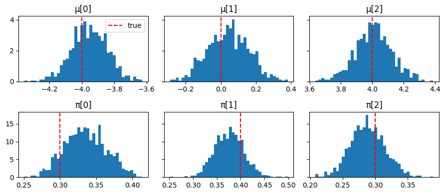
Posterior E[μ]: [-3.9499998  0.05       4.0099998]   true: [-4.  0.  4.]
Posterior E[π]: [0.32999998 0.38       0.29      ]   true: [0.3 0.4 0.3]
Mean acceptance rate: 0.90

Which approach to use

	Pure Funsor	NumPyro + Funsor
Model syntax	Explicit named-tensor algebra	numpyro.sample / numpyro.plate
Priors and transforms	Manual	Automatic
Discrete marginalisation	reduce(logaddexp, "z")	@config_enumerate + initialize_model
Requires NumPyro	No	Yes
Best for	Understanding Funsor internals	Production models, complex plate structure