Use with PyTensor models

Blackjax accepts any log-probability function as long as it is compatible with jax.jit, jax.grad (for gradient-based samplers) and jax.vmap. In this example we show how to use PyTensor as a modeling language and Blackjax as an inference library.

Before you start

You will need PyTensor to run this example.

pip install pytensor

```{note}
This notebook used to demonstrate Aesara integration.
Aesara has been archived and is incompatible with NumPy 2.x.
PyTensor is its actively-maintained successor with an almost identical API.

We implement the following Binomial response model for the rat tumor dataset:

$$ \begin{align*} Y &\sim \operatorname{Binomial}(N, \theta)\ \theta &\sim \operatorname{Beta}(\alpha, \beta)\ \alpha, \beta &\sim \frac{1}{(\alpha + \beta)^{2.5}} \end{align*} $$

We sample in the unconstrained space: \(\log\alpha\), \(\log\beta\), and \(\text{logit}(\theta)\).

Show code cell content

Hide code cell content

import numpy as np

# index of array is type of tumor and value shows number of total people tested.
group_size = np.array([20, 20, 20, 20, 20, 20, 20, 19, 19, 19, 19, 18, 18, 17, 20, 20, 20, 20, 19, 19, 18, 18, 25, 24, 23, 20, 20, 20, 20, 20, 20, 10, 49, 19, 46, 27, 17, 49, 47, 20, 20, 13, 48, 50, 20, 20, 20, 20, 20, 20, 20, 48, 19, 19, 19, 22, 46, 49, 20, 20, 23, 19, 22, 20, 20, 20, 52, 46, 47, 24, 14])
n_of_positives = np.array([0, 0, 0, 0, 0, 0, 0, 0, 0, 0, 0, 0, 0, 0, 1, 1, 1, 1, 1, 1, 1, 1, 2, 2, 2, 2, 2, 2, 2, 2, 2, 1, 5, 2, 5, 3, 2, 7, 7, 3, 3, 2, 9, 10, 4, 4, 4, 4, 4, 4, 4, 10, 4, 4, 4, 5, 11, 12, 5, 5, 6, 5, 6, 6, 6, 6, 16, 15, 15, 9, 4])
n_rat_tumors = len(group_size)

import jax
from datetime import date
rng_key = jax.random.key(int(date.today().strftime("%Y%m%d")))

We build the log-density graph symbolically in PyTensor. We work in the unconstrained space using \(\log\alpha\), \(\log\beta\), and \(\text{logit}(\theta_i)\) as free parameters and include the log-Jacobian corrections for the transforms:

import pytensor
import pytensor.tensor as pt
from pytensor.tensor.special import gammaln

log_a       = pt.scalar('log_a')
log_b       = pt.scalar('log_b')
logit_theta = pt.vector('logit_theta')

a     = pt.exp(log_a)
b     = pt.exp(log_b)
theta = pt.sigmoid(logit_theta)

# Improper prior: -2.5 * log(alpha + beta)
logprior_ab = -2.5 * pt.log(a + b)

# Log-Jacobians of the parameter transforms
logdet_a     = log_a
logdet_b     = log_b
logdet_theta = pt.sum(pt.log(theta) + pt.log(1 - theta))

# Beta(a, b) log-density for each theta_i
logp_beta = pt.sum(
    gammaln(a + b) - gammaln(a) - gammaln(b)
    + (a - 1) * pt.log(theta)
    + (b - 1) * pt.log(1 - theta)
)

# Binomial log-likelihood
logp_binom = pt.sum(
    n_of_positives * pt.log(theta)
    + (group_size - n_of_positives) * pt.log(1 - theta)
)

logdensity = logprior_ab + logdet_a + logdet_b + logdet_theta + logp_beta + logp_binom

To sample with Blackjax we compile the log-density graph using PyTensor’s JAX backend, which produces a function fully compatible with jax.jit and jax.grad:

fn_jax  = pytensor.function([log_a, log_b, logit_theta], logdensity, mode="JAX")
jit_fn  = fn_jax.vm.jit_fn   # the underlying JAX function

def logdensity_fn(position):
    """Wrap positional args into a dict-compatible interface for Blackjax."""
    return jit_fn(position["log_a"], position["log_b"], position["logit_theta"])[0]

Let’s define the initial position and run window adaptation for the NUTS sampler:

import blackjax

def init_param_fn(seed):
    key1, key2, key3 = jax.random.split(seed, 3)
    return {
        "log_a":       jax.random.normal(key1, ()),
        "log_b":       jax.random.normal(key2, ()),
        "logit_theta": jax.random.normal(key3, (n_rat_tumors,)),
    }

rng_key, init_key, warmup_key, sample_key = jax.random.split(rng_key, 4)
init_position = init_param_fn(init_key)

adapt = blackjax.window_adaptation(blackjax.nuts, logdensity_fn)
(state, parameters), _ = adapt.run(warmup_key, init_position, 1000)
kernel = blackjax.nuts(logdensity_fn, **parameters).step

Now we run the inference loop:

Show code cell content

Hide code cell content

def inference_loop(rng_key, kernel, initial_state, num_samples):
    @jax.jit
    def one_step(state, rng_key):
        state, infos = kernel(rng_key, state)
        return state, (state, infos)

    keys = jax.random.split(rng_key, num_samples)
    _, (states, infos) = jax.lax.scan(one_step, initial_state, keys)
    return states, infos

states, infos = inference_loop(sample_key, kernel, state, 1000)

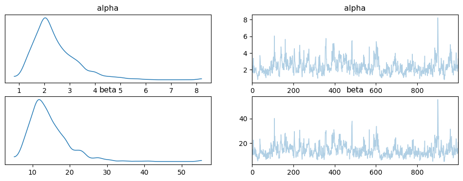
And plot the posterior samples on the original (constrained) scale using ArviZ:

import numpy as np
import arviz as az

posterior = {
    "alpha": np.exp(states.position["log_a"]),
    "beta":  np.exp(states.position["log_b"]),
}
idata = az.from_dict(posterior={k: v[None, ...] for k, v in posterior.items()})
az.plot_trace(idata);