Use Tempered SMC to Improve Exploration of MCMC Methods.

Multimodal distributions are typically hard to sample from, in particular using energy based methods such as HMC, as you need high energy levels to escape a potential well.

Tempered SMC helps with this by considering a sequence of distributions:

\[ p_{\lambda_k}(x) \propto p_0(x) \exp(-\lambda_k V(x)) \]

where the tempering parameter \(\lambda_k\) takes increasing values between \(0\) and \(1\). Tempered SMC will also particularly shine when the MCMC step is not well calibrated (too small step size, etc) like in the example below.

Imports

Show code cell content Hide code cell content

import matplotlib.pyplot as plt

plt.rcParams["axes.spines.right"] = False
plt.rcParams["axes.spines.top"] = False

import jax

from datetime import date
rng_key = jax.random.key(int(date.today().strftime("%Y%m%d")))

import numpy as np
import jax.numpy as jnp
from jax.scipy.stats import multivariate_normal

import blackjax
import blackjax.smc.resampling as resampling
from blackjax.smc import extend_params

Sampling From a Bimodal Potential

Experimental Setup

We consider a prior distribution

\[ p_0(x) = \mathcal{N}(x \mid 0, 1) \]

and a potential function

\[ V(x) = (x^2 - 1)^2 \]

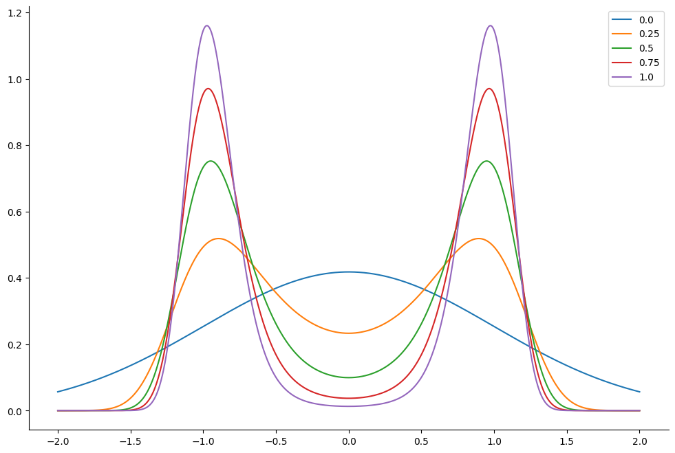
This corresponds to the following distribution. We plot the resulting tempered density for 5 different values of \(\lambda_k\) : from \(\lambda_k =1\) which correponds to the original density to \(\lambda_k=0\). The lower the value of \(\lambda_k\) the easier it is for the sampler to jump between the modes of the posterior density.

def V(x):
    return 5 * jnp.square(jnp.sum(x**2, axis=-1) - 1)


def prior_log_prob(x):
    d = x.shape[-1]
    return multivariate_normal.logpdf(x, jnp.zeros((d,)), jnp.eye(d))


linspace = jnp.linspace(-2, 2, 5000)[..., None]
lambdas = jnp.linspace(0.0, 1.0, 5)
prior_logvals = prior_log_prob(linspace)
potential_vals = V(linspace)
log_res = prior_logvals - lambdas[..., None] * potential_vals

density = jnp.exp(log_res)
normalizing_factor = jnp.sum(density, axis=1, keepdims=True) * (
    linspace[1] - linspace[0]
)
density /= normalizing_factor

Show code cell source Hide code cell source

fig, ax = plt.subplots(figsize=(12, 8))
ax.plot(linspace.squeeze(), density.T)
ax.legend(list(lambdas));

def inference_loop(rng_key, mcmc_kernel, initial_state, num_samples):
    @jax.jit
    def one_step(state, k):
        state, _ = mcmc_kernel(k, state)
        return state, state

    keys = jax.random.split(rng_key, num_samples)
    _, states = jax.lax.scan(one_step, initial_state, keys)

    return states


def full_logdensity(x):
    return -V(x) + prior_log_prob(x)


inv_mass_matrix = jnp.eye(1)
n_samples = 10_000

Sample with HMC

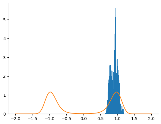
We first try to sample from the posterior density using an HMC kernel.

%%time

hmc_parameters = dict(
    step_size=1e-4, inverse_mass_matrix=inv_mass_matrix, num_integration_steps=50
)

hmc = blackjax.hmc(full_logdensity, **hmc_parameters)
hmc_state = hmc.init(jnp.ones((1,)))

rng_key, sample_key = jax.random.split(rng_key)
hmc_samples = inference_loop(sample_key, hmc.step, hmc_state, n_samples)

CPU times: user 1.13 s, sys: 101 ms, total: 1.24 s
Wall time: 1.23 s

Show code cell source Hide code cell source

samples = np.array(hmc_samples.position[:, 0])
_ = plt.hist(samples, bins=100, density=True)
_ = plt.plot(linspace.squeeze(), density[-1])

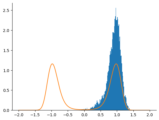
Sample with NUTS

We now use a NUTS kernel.

%%time

nuts_parameters = dict(step_size=1e-4, inverse_mass_matrix=inv_mass_matrix)

nuts = blackjax.nuts(full_logdensity, **nuts_parameters)
nuts_state = nuts.init(jnp.ones((1,)))

rng_key, sample_key = jax.random.split(rng_key)
nuts_samples = inference_loop(sample_key, nuts.step, nuts_state, n_samples)

CPU times: user 5.01 s, sys: 58.7 ms, total: 5.06 s
Wall time: 5.05 s

Show code cell source Hide code cell source

samples = np.array(nuts_samples.position[:, 0])
_ = plt.hist(samples, bins=100, density=True)
_ = plt.plot(linspace.squeeze(), density[-1])

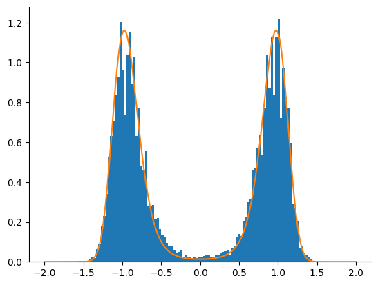
Tempered SMC with HMC Kernel

We now use the adaptive tempered SMC algorithm with an HMC kernel. We only take one HMC step before resampling. The algorithm is run until \(\lambda_k\) crosses the \(\lambda_k = 1\) limit.

def smc_inference_loop(rng_key, smc_kernel, initial_state):
    """Run the temepered SMC algorithm.

    We run the adaptive algorithm until the tempering parameter lambda reaches the value
    lambda=1.

    """

    def cond(carry):
        i, state, _k = carry
        return state.lmbda < 1

    def one_step(carry):
        i, state, k = carry
        k, subk = jax.random.split(k, 2)
        state, _ = smc_kernel(subk, state)
        return i + 1, state, k

    n_iter, final_state, _ = jax.lax.while_loop(
        cond, one_step, (0, initial_state, rng_key)
    )

    return n_iter, final_state

%%time

loglikelihood = lambda x: -V(x)

hmc_parameters = dict(
    step_size=1e-4, inverse_mass_matrix=inv_mass_matrix, num_integration_steps=1
)

tempered = blackjax.adaptive_tempered_smc(
    prior_log_prob,
    loglikelihood,
    blackjax.hmc.build_kernel(),
    blackjax.hmc.init,
    extend_params(n_samples, hmc_parameters),
    resampling.systematic,
    0.5,
    num_mcmc_steps=1,
)

rng_key, init_key, sample_key = jax.random.split(rng_key, 3)
initial_smc_state = jax.random.multivariate_normal(
    init_key, jnp.zeros([1]), jnp.eye(1), (n_samples,)
)
initial_smc_state = tempered.init(initial_smc_state)

n_iter, smc_samples = smc_inference_loop(sample_key, tempered.step, initial_smc_state)
print("Number of steps in the adaptive algorithm: ", n_iter.item())

Number of steps in the adaptive algorithm:  11
CPU times: user 2.57 s, sys: 433 ms, total: 3 s
Wall time: 2.64 s

Show code cell source Hide code cell source

samples = np.array(smc_samples.particles[:, 0])
_ = plt.hist(samples, bins=100, density=True)
_ = plt.plot(linspace.squeeze(), density[-1])

Sampling from the Rastrigin Potential

Experimental Setup

We consider a prior distribution \(p_0(x) = \mathcal{N}(x \mid 0_2, 2 I_2)\) and we want to sample from a Rastrigin type potential function \(V(x) = -2 A + \sum_{i=1}^2x_i^2 - A \cos(2 \pi x_i)\) where we choose \(A=10\). These potential functions are known to be particularly hard to sample.

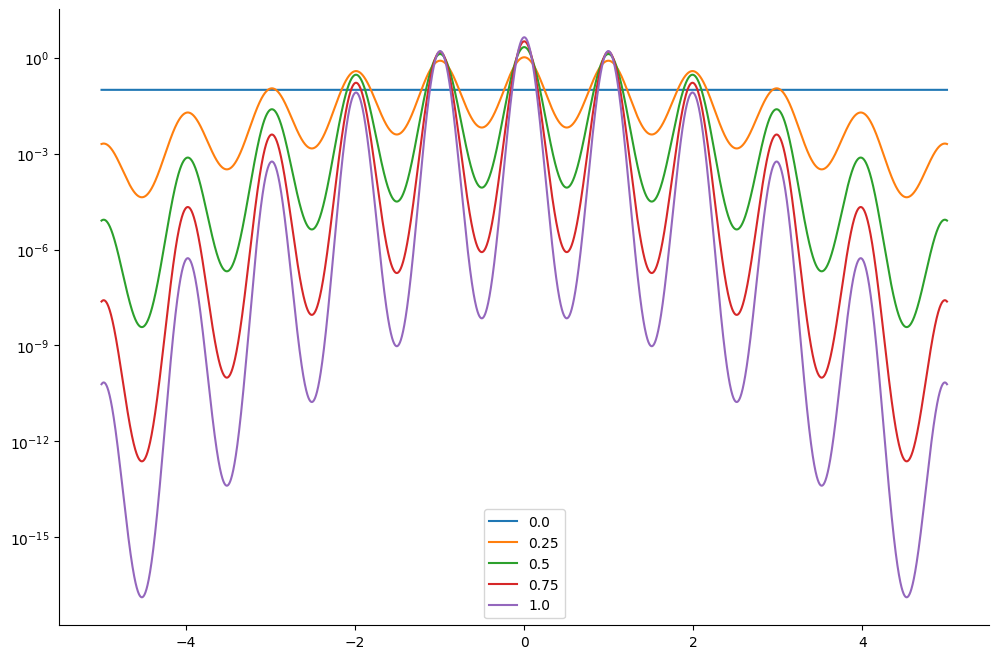
We plot the resulting tempered density for 5 different values of \(\lambda_k\): from \(\lambda_k =1\) which correponds to the original density to \(\lambda_k=0\). The lower the value of \(\lambda_k\) the easier it is to sampler from the posterior log-density.

def V(x):
    d = x.shape[-1]
    res = -10 * d + jnp.sum(x**2 - 10 * jnp.cos(2 * jnp.pi * x), -1)
    return res


linspace = jnp.linspace(-5, 5, 5000)[..., None]
lambdas = jnp.linspace(0.0, 1.0, 5)
potential_vals = V(linspace)
log_res = lambdas[..., None] * potential_vals

density = jnp.exp(-log_res)
normalizing_factor = jnp.sum(density, axis=1, keepdims=True) * (
    linspace[1] - linspace[0]
)
density /= normalizing_factor

Show code cell source Hide code cell source

fig, ax = plt.subplots(figsize=(12, 8))
ax.semilogy(linspace.squeeze(), density.T)
ax.legend(list(lambdas))

<matplotlib.legend.Legend at 0x7f14007be810>

def inference_loop(rng_key, mcmc_kernel, initial_state, num_samples):
    def one_step(state, k):
        state, _ = mcmc_kernel(k, state)
        return state, state

    keys = jax.random.split(rng_key, num_samples)
    _, states = jax.lax.scan(one_step, initial_state, keys)

    return states


inv_mass_matrix = jnp.eye(1)
n_samples = 1_000

HMC Sampler

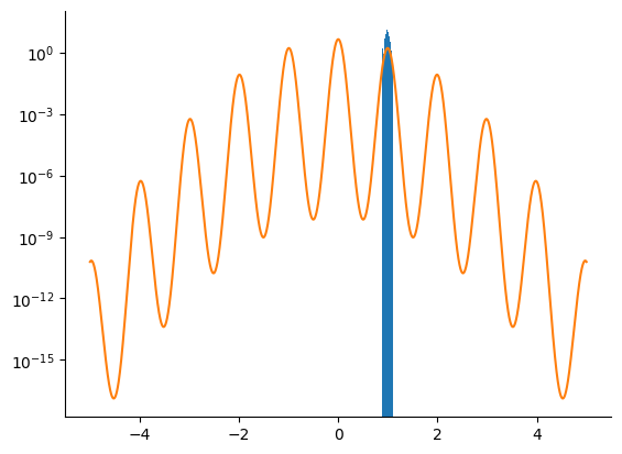
We first try to sample from the posterior density using an HMC kernel.

%%time

loglikelihood = lambda x: -V(x)

hmc_parameters = dict(
    step_size=1e-2, inverse_mass_matrix=inv_mass_matrix, num_integration_steps=50
)

hmc = blackjax.hmc(full_logdensity, **hmc_parameters)
hmc_state = hmc.init(jnp.ones((1,)))

rng_key, sample_key = jax.random.split(rng_key)
hmc_samples = inference_loop(sample_key, hmc.step, hmc_state, n_samples)

CPU times: user 564 ms, sys: 35.4 ms, total: 599 ms
Wall time: 592 ms

Show code cell source Hide code cell source

samples = np.array(hmc_samples.position[:, 0])
_ = plt.hist(samples, bins=100, density=True)
_ = plt.plot(linspace.squeeze(), density[-1])
_ = plt.yscale("log")

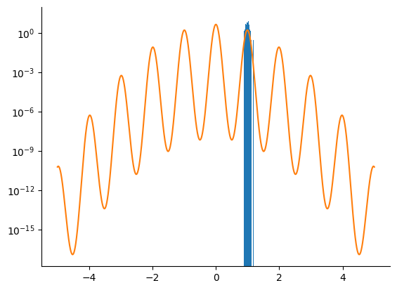
NUTS Sampler

We do the same using a NUTS kernel.

%%time

nuts_parameters = dict(step_size=1e-2, inverse_mass_matrix=inv_mass_matrix)

nuts = blackjax.nuts(full_logdensity, **nuts_parameters)
nuts_state = nuts.init(jnp.ones((1,)))

rng_key, sample_key = jax.random.split(rng_key)
nuts_samples = inference_loop(sample_key, nuts.step, nuts_state, n_samples)

CPU times: user 887 ms, sys: 48 ms, total: 935 ms
Wall time: 923 ms

Show code cell source Hide code cell source

samples = np.array(nuts_samples.position[:, 0])
_ = plt.hist(samples, bins=100, density=True)
_ = plt.plot(linspace.squeeze(), density[-1])
_ = plt.yscale("log")

Tempered SMC with HMC Kernel

We now use the adaptive tempered SMC algorithm with an HMC kernel. We only take one HMC step before resampling. The algorithm is run until \(\lambda_k\) crosses the \(\lambda_k = 1\) limit. We correct the bias introduced by the (arbitrary) prior.

%%time

loglikelihood = lambda x: -V(x)

hmc_parameters = dict(
    step_size=1e-2, inverse_mass_matrix=inv_mass_matrix, num_integration_steps=100
)

tempered = blackjax.adaptive_tempered_smc(
    prior_log_prob,
    loglikelihood,
    blackjax.hmc.build_kernel(),
    blackjax.hmc.init,
    extend_params(n_samples, hmc_parameters),
    resampling.systematic,
    0.75,
    num_mcmc_steps=1,
)

rng_key, init_key, sample_key = jax.random.split(rng_key, 3)
initial_smc_state = jax.random.multivariate_normal(
    init_key, jnp.zeros([1]), jnp.eye(1), (n_samples,)
)
initial_smc_state = tempered.init(initial_smc_state)

n_iter, smc_samples = smc_inference_loop(sample_key, tempered.step, initial_smc_state)
print("Number of steps in the adaptive algorithm: ", n_iter.item())

Number of steps in the adaptive algorithm:  9
CPU times: user 1.93 s, sys: 114 ms, total: 2.04 s
Wall time: 2.02 s

Show code cell source Hide code cell source

samples = np.array(smc_samples.particles[:, 0])
_ = plt.hist(samples, bins=100, density=True)
_ = plt.plot(linspace.squeeze(), density[-1])
_ = plt.yscale("log")

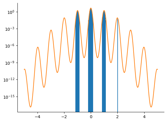
The tempered SMC algorithm with the HMC kernel clearly outperfoms the HMC and NUTS kernels alone.