Cyclical SGLD

Cyclical SGLD#

In this example we will demonstrate how Blackjax can be used to create non-trivial samplers by implementing Cyclical SGLD [ZLZ+19]. Stochastic Gradient MCMC algorithms are typically used to sample from the posterior distribution of Bayesian Neural Networks. They differ from other gradient-based MCMC algorithms in that they estimate the gradient with minibatches of data instead of the full dataset.

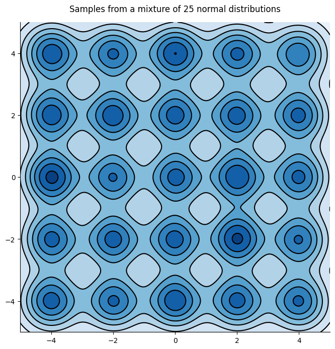
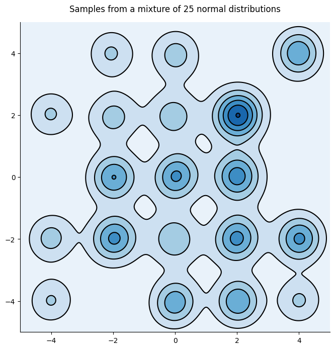
However, SGMCMC algorithms are inefficient at exploring multimodal distributions which are typical of neural networks. To see this let’s consider a simple yet challenging example, an array of 25 gaussian distributions:

import jax

from datetime import date
rng_key = jax.random.key(int(date.today().strftime("%Y%m%d")))

import numpy as np
import jax.scipy as jsp
import jax.numpy as jnp


positions = np.asarray([-4, -2, 0, 2, 4], dtype=np.float32)
mu = np.asarray(np.meshgrid(positions, positions)).reshape(2, -1).T
lmbda = 1 / mu.shape[0]
sigma = 0.03 * jnp.eye(2)


def logprob_fn(x, *_):
    return jnp.sum(
        jnp.log(lmbda)
        + jsp.special.logsumexp(
            jax.scipy.stats.multivariate_normal.logpdf(x, mu, sigma), axis=-1
        )
    )


def sample_fn(rng_key):
    choose_key, sample_key = jax.random.split(rng_key)
    samples = jax.random.multivariate_normal(sample_key, mu, sigma)
    return jax.random.choice(choose_key, samples)

../_images/28c7c65a25398d155fa615e26bd8eae176dff4f90b4954a8978c2a5d88f5dbc0.png

SGLD#

Let us build a SGLD sampler with Blackjax with a decreading learning rate, and generate samples from this distribution:

import blackjax
from fastprogress import progress_bar


# 50k iterations
num_training_steps = 50000
schedule_fn = lambda k: 0.05 * k ** (-0.55)
schedule = schedule_fn(np.arange(1, num_training_steps+1))

grad_fn = lambda x, _: jax.grad(logprob_fn)(x)
sgld = blackjax.sgld(grad_fn)

rng_key, init_key = jax.random.split(rng_key)
init_position = -10 + 20 * jax.random.uniform(init_key, shape=(2,))

position = sgld.init(init_position)
sgld_samples = []
for i in progress_bar(range(num_training_steps)):
    rng_key, sample_key = jax.random.split(rng_key)
    position = jax.jit(sgld.step)(sample_key, position, 0, schedule[i])
    sgld_samples.append(position)
sgld_samples = np.asarray(sgld_samples)

100.00% [50000/50000 00:11<00:00]

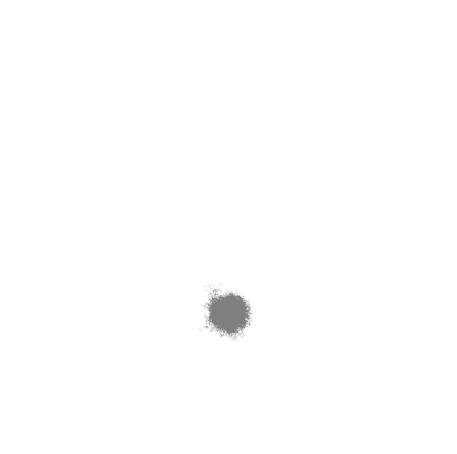
As one can see on the following figure, SGLD has a hard time escaping the mode in which it started, leading to a poor approximation of the distribution:

../_images/2715a2d00fd0904832a7349c6e2de7453cd2b97318eebcdef04c33040df8e8fd.png

Cyclical SGLD#

To escape modes and better explore distributions, Cyclical SLGD alternes between two phases:

Exploration using Stochastic Gradient Descent with a large-ish step size;
Sampling using SGLD with a lower learning rate.

Cyclical schedule#

Both the step size and the phase the algorithm is in are governed by a cyclical schedule which is built as follows:

from typing import NamedTuple


class ScheduleState(NamedTuple):
    step_size: float
    do_sample: bool


def build_schedule(
    num_training_steps,
    num_cycles=4,
    initial_step_size=1e-3,
    exploration_ratio=0.25,
):
    cycle_length = num_training_steps // num_cycles

    def schedule_fn(step_id):
        do_sample = False
        if ((step_id % cycle_length)/cycle_length) >= exploration_ratio:
            do_sample = True

        cos_out = jnp.cos(jnp.pi * (step_id % cycle_length) / cycle_length) + 1
        step_size = 0.5 * cos_out * initial_step_size

        return ScheduleState(step_size, do_sample)

    return schedule_fn

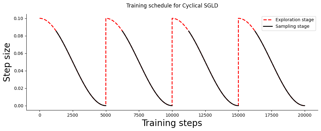
Let us visualize a schedule for 200k training steps divided in 4 cycles. At each cycle 1/4th of the steps are dedicated to exploration:

../_images/5436d9272b3f1e7b548a0d5d7203da5ed14fc3d2c07520835d4b46c1d3940f91.png

Step function#

Let us now build a step function for the Cyclical SGLD algorithm that can act as a drop-in replacement to the SGLD kernel.

import optax

from blackjax.types import ArrayTree
from optax._src.base import OptState


class CyclicalSGMCMCState(NamedTuple):
    """State of the Cyclical SGMCMC sampler.
    """
    position: ArrayTree
    opt_state: OptState


def cyclical_sgld(grad_estimator_fn, loglikelihood_fn):

    # Initialize the SgLD step function
    sgld = blackjax.sgld(grad_estimator_fn)
    sgd = optax.sgd(1.)

    def init_fn(position):
        opt_state = sgd.init(position)
        return CyclicalSGMCMCState(position, opt_state)

    def step_fn(rng_key, state, minibatch, schedule_state):
        """Cyclical SGLD kernel."""

        def step_with_sgld(current_state):
            rng_key, state, minibatch, step_size = current_state
            new_position = sgld.step(rng_key, state.position, minibatch, step_size)
            return CyclicalSGMCMCState(new_position, state.opt_state)

        def step_with_sgd(current_state):
            _, state, minibatch, step_size = current_state
            grads = grad_estimator_fn(state.position, 0)
            rescaled_grads = - 1. * step_size * grads
            updates, new_opt_state = sgd.update(
                rescaled_grads, state.opt_state, state.position
                )
            new_position = optax.apply_updates(state.position, updates)
            return CyclicalSGMCMCState(new_position, new_opt_state)

        new_state = jax.lax.cond(
            schedule_state.do_sample,
            step_with_sgld,
            step_with_sgd,
            (rng_key, state, minibatch, schedule_state.step_size)
        )

        return new_state

    return init_fn, step_fn

We leave the implementation of Cyclical SGHMC as an exercise for the reader.

Note

If you want to Cyclical SGLD on one of your models you can simply copy and paste the code in the above cell and the cell where the schedule builder is implemented.

Let’s sample using Cyclical SGLD, for the same number of iterations as with SGLD. We’ll use 30 cycles, and sample 75% of the time.

# 50k iterations
# M = 30
# initial step size = 0.09
# ratio exploration = 1/4
num_training_steps = 50000
schedule_fn = build_schedule(num_training_steps, 30, 0.09, 0.25)
schedule = [schedule_fn(i) for i in range(num_training_steps)]

grad_fn = lambda x, _: jax.grad(logprob_fn)(x)
init, step = cyclical_sgld(grad_fn, logprob_fn)

rng_key, init_key = jax.random.split(rng_key)
init_position = -10 + 20 * jax.random.uniform(init_key, shape=(2,))
init_state = init(init_position)


state = init_state
cyclical_samples = []
for i in progress_bar(range(num_training_steps)):
    rng_key, sample_key = jax.random.split(rng_key)
    state = jax.jit(step)(sample_key, state, 0, schedule[i])
    if schedule[i].do_sample:
        cyclical_samples.append(state.position)

cyclical_samples = np.asarray(cyclical_samples)

100.00% [50000/50000 00:11<00:00]

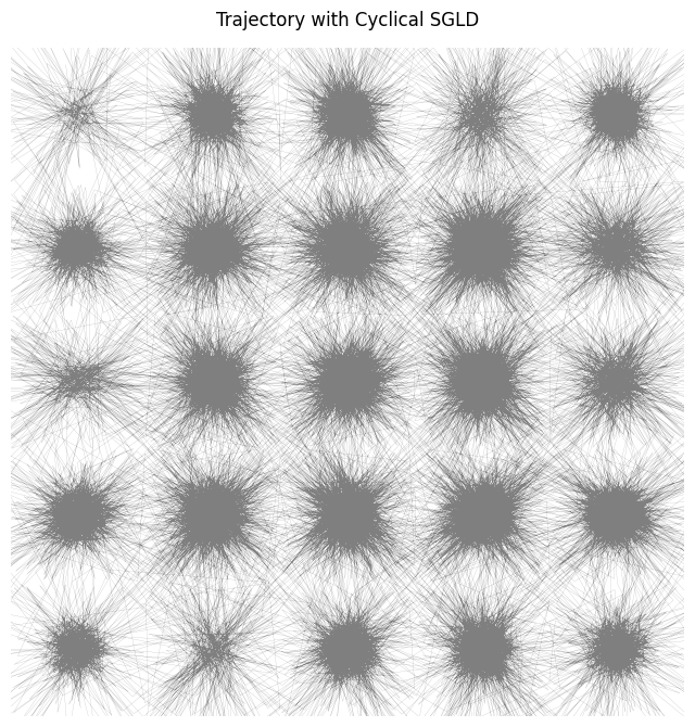
By looking at the trajectory of the sampler it seems that the distribution is much better explored:

../_images/db8af4e6c294e0e160568e0574936a4a25c5a05222f3b5ac75c0b2a9f0ab5530.png

And the distribution indeed looks more better:

../_images/7627b75dc2127e8226d09b683e7f713bc8b7a4fac62e9d7dacb2793dd8dd1255.png

Warning

SciPy’s gaussian_kde assumes that the total number of points provided is the sample size, it is thus not fit to use with raw MCMC samples. We should instead pass the bandwidth manually \(n_{eff}^{-1/6}\) where \(n_{eff}\) is the effective number of samples, and the figure should capture more modes.

[ZLZ+19]

Ruqi Zhang, Chunyuan Li, Jianyi Zhang, Changyou Chen, and Andrew Gordon Wilson. Cyclical stochastic gradient mcmc for bayesian deep learning. In International Conference on Learning Representations. 2019.

Cyclical SGLD

Contents

Cyclical SGLD#

SGLD#

Cyclical SGLD#

Cyclical schedule#

Step function#