Bayesian Logistic Regression

In this notebook we demonstrate the use of the random walk Rosenbluth-Metropolis-Hasting algorithm on a simple logistic regression.

Show code cell content Hide code cell content

import matplotlib.pyplot as plt

plt.rcParams["axes.spines.right"] = False
plt.rcParams["axes.spines.top"] = False
plt.rcParams["figure.figsize"] = (12, 8)

import jax

from datetime import date
rng_key = jax.random.key(int(date.today().strftime("%Y%m%d")))

import jax.numpy as jnp
from sklearn.datasets import make_biclusters

import blackjax

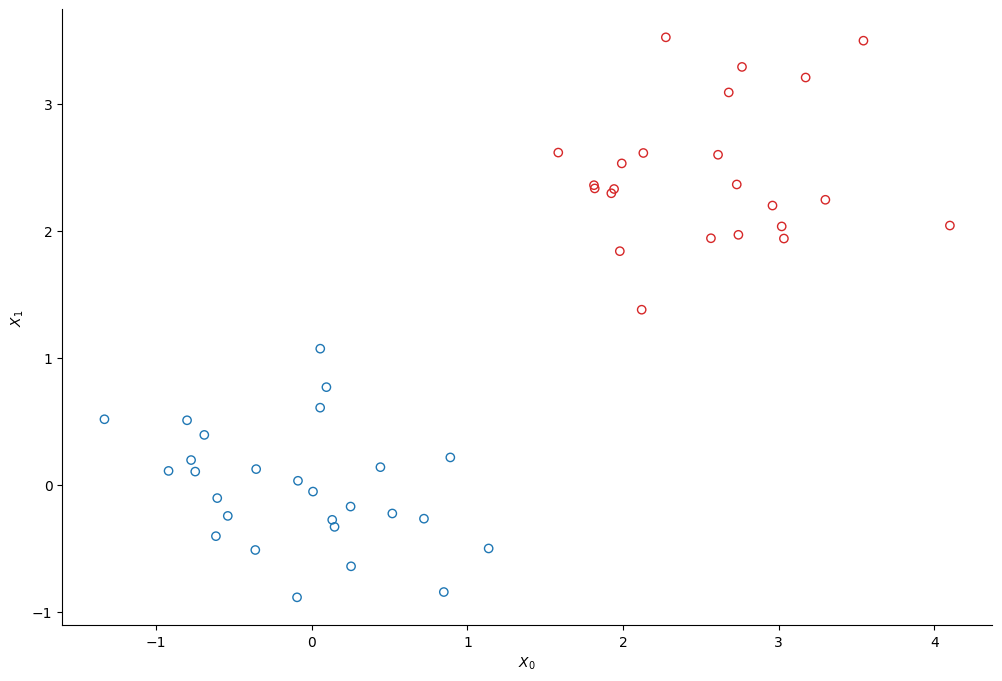
The Data

We create two clusters of points using scikit-learn’s make_bicluster function.

num_points = 50
X, rows, cols = make_biclusters(
    (num_points, 2), 2, noise=0.6, random_state=314, minval=-3, maxval=3
)
y = rows[0] * 1.0  # y[i] = whether point i belongs to cluster 1

Show code cell source Hide code cell source

colors = ["tab:red" if el else "tab:blue" for el in rows[0]]
plt.scatter(*X.T, edgecolors=colors, c="none")
plt.xlabel(r"$X_0$")
plt.ylabel(r"$X_1$");

The Model

We use a simple logistic regression model to infer to which cluster each of the points belongs. We note \(y\) a binary variable that indicates whether a point belongs to the first cluster :

\[ y \sim \operatorname{Bernoulli}(p) \]

The probability \(p\) to belong to the first cluster commes from a logistic regression:

\[ p = \operatorname{logistic}(\Phi\,\boldsymbol{w}) \]

where \(w\) is a vector of weights whose priors are a normal prior centered on 0:

\[ \boldsymbol{w} \sim \operatorname{Normal}(0, \sigma) \]

And \(\Phi\) is the matrix that contains the data, so each row \(\Phi_{i,:}\) is the vector \(\left[1, X_0^i, X_1^i\right]\)

Phi = jnp.c_[jnp.ones(num_points)[:, None], X]
N, M = Phi.shape


def sigmoid(z):
    return jnp.exp(z) / (1 + jnp.exp(z))


def log_sigmoid(z):
    return z - jnp.log(1 + jnp.exp(z))


def logdensity_fn(w, alpha=1.0):
    """The log-probability density function of the posterior distribution of the model."""
    log_an = log_sigmoid(Phi @ w)
    an = Phi @ w
    log_likelihood_term = y * log_an + (1 - y) * jnp.log(1 - sigmoid(an))
    prior_term = alpha * w @ w / 2

    return -prior_term + log_likelihood_term.sum()

Posterior Sampling

We use blackjax’s Random Walk RMH kernel to sample from the posterior distribution.

rng_key, init_key = jax.random.split(rng_key)

w0 = jax.random.multivariate_normal(init_key, 0.1 + jnp.zeros(M), jnp.eye(M))
rmh = blackjax.rmh(logdensity_fn, blackjax.mcmc.random_walk.normal(jnp.ones(M) * 0.05))
initial_state = rmh.init(w0)

Since blackjax does not provide an inference loop we need to implement one ourselves:

def inference_loop(rng_key, kernel, initial_state, num_samples):
    @jax.jit
    def one_step(state, rng_key):
        state, _ = kernel(rng_key, state)
        return state, state

    keys = jax.random.split(rng_key, num_samples)
    _, states = jax.lax.scan(one_step, initial_state, keys)

    return states

We can now run the inference:

rng_key, sample_key = jax.random.split(rng_key)
states = inference_loop(sample_key, rmh.step, initial_state, 5_000)

And display the trace:

Show code cell source Hide code cell source

burnin = 300

fig, ax = plt.subplots(1, 3, figsize=(12, 2))
for i, axi in enumerate(ax):
    axi.plot(states.position[:, i])
    axi.set_title(f"$w_{i}$")
    axi.axvline(x=burnin, c="tab:red")
plt.show()

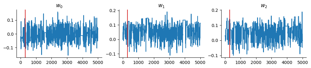
burnin = 300
chains = states.position[burnin:, :]
nsamp, _ = chains.shape

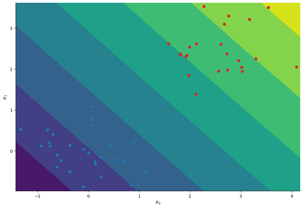
Predictive Distribution

Having infered the posterior distribution of the regression’s coefficients we can compute the probability to belong to the first cluster at each position \((X_0, X_1)\).

# Create a meshgrid
xmin, ymin = X.min(axis=0) - 0.1
xmax, ymax = X.max(axis=0) + 0.1
step = 0.1
Xspace = jnp.mgrid[xmin:xmax:step, ymin:ymax:step]
_, nx, ny = Xspace.shape

# Compute the average probability to belong to the first cluster at each point on the meshgrid
Phispace = jnp.concatenate([jnp.ones((1, nx, ny)), Xspace])
Z_mcmc = sigmoid(jnp.einsum("mij,sm->sij", Phispace, chains))
Z_mcmc = Z_mcmc.mean(axis=0)

Show code cell source Hide code cell source

plt.contourf(*Xspace, Z_mcmc)
plt.scatter(*X.T, c=colors)
plt.xlabel(r"$X_0$")
plt.ylabel(r"$X_1$");