Bayesian Regression With Latent Gaussian Sampler#
In this example, we want to illustrate how to use the marginal sampler implementation mgrad_gaussian of the article Auxiliary gradient-based sampling algorithms [TP18]. We do so by using the simulated data from the example Gaussian Regression with the Elliptical Slice Sampler. Please also refer to the complementary example Bayesian Logistic Regression With Latent Gaussian Sampler.
Sampler Overview#
In section we give a brief overview of the idea behind this particular sampler. For more details please refer to the original paper Auxiliary gradient-based sampling algorithms (here you can access the arXiv preprint).
Motivation: Auxiliary Metropolis-Hastings samplers#
Let us recall how to sample from a target density \(\pi(\mathbf{x})\) using a Metropolis-Hasting sampler trough a marginal scheme process. The main idea is to have a mechanism that generate proposals \(y\) which we then accept or reject according to a specific criterion. Concretely, suppose that we have an auxiliary scheme given by
Sample \(\mathbf{u}|\mathbf{x} \sim \pi(\mathbf{u}|\mathbf{x}) = q(\mathbf{u}|\mathbf{x})\).
Generate proposal \(\mathbf{y}|\mathbf{u}, \mathbf{x} \sim q(\mathbf{y}|\mathbf{x}, \mathbf{u})\)
Compute the Metropolis-Hasting ratio
Accept proposal \(y\) with probability \(\min(1, \tilde{\varrho})\) and reject it otherwise.
This scheme targets the auxiliary distribution \(\pi(\mathbf{x}, \mathbf{u}) = \pi(\mathbf{x}) q(\mathbf{u}|\mathbf{x})\) in two steps.
Now, suppose we can instead compute the marginal proposal distribution \(q(\mathbf{y}|\mathbf{x}) = \int q(\mathbf{y}|\mathbf{x}, \mathbf{u}) q(\mathbf{u}|\mathbf{x}) \mathrm{d}u\) in closed form, then an alternative scheme is given by:
We draw a proposal \(y \sim q(\mathbf{y}\mid\mathbf{x})\).
Then we compute the Metropolis-Hasting ratio
Accept proposal \(y\) with probability \(\min(1, \varrho)\) and reject it otherwise.
Example: Auxiliary Metropolis-Adjusted Langevin Algorithm (MALA)#
Let’s consider the case of an auxiliary random walk proposal \(q(\mathbf{u}|\mathbf{x}) = N(\mathbf{u}|\mathbf{x}, (\delta /2) \mathbf{I})\) for \(\delta > 0\) as in [Section 2.2] Auxiliary gradient-based sampling algorithms, it is shown that one can use a first order approximation to sample from the (intractable) \(\pi(\mathbf{x}|\mathbf{u})\) density by choosing
The resulting marginal sampler can be shown to correspond to the Metropolis-adjusted Langevin algorithm (MALA) with
Latent Gaussian Models#
A particular case of interest is the latent Gaussian model where the target density has the form
In this case, instead of linearising the full log density \(\log \pi(\mathbf{x})\), we can linearise \(f\) only, which, when combined with a random walk proposal \(N(\mathbf{u}|\mathbf{x}, (\delta /2) \mathbf{I})\), recovers to the following auxiliary proposal
where \(\mathbf{A} = \delta / 2(\mathbf{C} + (\delta / 2)\mathbf{I})^{-1}\mathbf{C}\). The corresponding marginal density is
Sampling from \(\pi(\mathbf{x}, \mathbf{u})\), and therefore from \(\pi(\mathbf{x})\), is done via Hastings-within-Gibbs as above.
A crucial point of this algorithm is the fact that \(\mathbf{A}\) can be precomputed and afterward modified cheaply when \(\delta\) varies. This makes it easy to calibrate the step-size \(\delta\) at low cost.
Now that we have a high-level understanding of the algorithm, let’s see how to use it in blackjax.
import jax

from datetime import date

rng_key = jax.random.key(int(date.today().strftime("%Y%m%d")))
import jax.numpy as jnp
import numpy as np

from blackjax import mgrad_gaussian
We generate data through a squared exponential kernel as in the example Gaussian Regression with the Elliptical Slice Sampler.
def squared_exponential(x, y, length, scale):
    dot_diff = jnp.dot(x, x) + jnp.dot(y, y) - 2 * jnp.dot(x, y)
    return scale**2 * jnp.exp(-0.5 * dot_diff / length**2)
n, d = 2000, 2
length, scale = 1.0, 1.0
y_sd = 1.0

# fake data
rng_key, kX, kf, ky = jax.random.split(rng_key, 4)

X = jax.random.uniform(kX, shape=(n, d))
Sigma = jax.vmap(
    lambda x: jax.vmap(lambda y: squared_exponential(x, y, length, scale))(X)
)(X) + 1e-3 * jnp.eye(n)
invSigma = jnp.linalg.inv(Sigma)
f = jax.random.multivariate_normal(kf, jnp.zeros(n), Sigma)
y = f + jax.random.normal(ky, shape=(n,)) * y_sd

# conjugate results
posterior_cov = jnp.linalg.inv(invSigma + 1 / y_sd**2 * jnp.eye(n))
posterior_mean = jnp.dot(posterior_cov, y) * 1 / y_sd**2
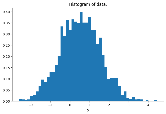
Let’s visualize the distribution of the vector y.
Sampling#
Now we proceed to run the sampler. First, we set the sampler parameters:
# sampling parameters
n_warm = 2000
n_iter = 500
Next, we define the the log-probability function. For this we need to set the log-likelihood function.
loglikelihood_fn = lambda f: -0.5 * jnp.dot(y - f, y - f) / y_sd**2
logdensity_fn = lambda f: loglikelihood_fn(f) - 0.5 * jnp.dot(f @ invSigma, f)
Now we are ready to initialize the sampler. The output is type is a NamedTuple with the following fields:
init:
    A pure function which when called with the initial position and the
    target density probability function will return the kernel's initial
    state.

step:
    A pure function that takes a rng key, a state and possibly some
    parameters and returns a new state and some information about the
    transition.
init, kernel = mgrad_gaussian(
    logdensity_fn=logdensity_fn, mean=jnp.zeros(n), covariance=Sigma, step_size=0.5
)
We continue by setting the inference loop.
def inference_loop(rng, init_state, kernel, n_iter):
    keys = jax.random.split(rng, n_iter)

    def step(state, key):
        state, info = kernel(key, state)
        return state, (state, info)

    _, (states, info) = jax.lax.scan(step, init_state, keys)
    return states, info
We are now ready to run the sampler! The only extra parameters in the step function is delta, which (as seen in the sampler description) corresponds (in a loose sense) to the step-size of MALA algorithm.
Adaptation
Note that one can calibrate the delta parameter as described in the example Bayesian Logistic Regression With Latent Gaussian Sampler.
%%time

initial_state = init(f)
rng_key, sample_key = jax.random.split(rng_key, 2)
states, info = inference_loop(sample_key, init(f), kernel, n_warm + n_iter)
samples = states.position[n_warm:]
CPU times: user 4.9 s, sys: 118 ms, total: 5.02 s
Wall time: 1.6 s
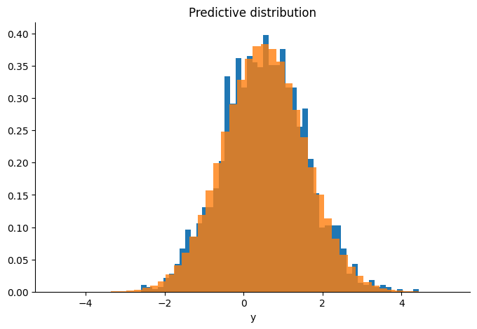
Diagnostics#
Finally we evaluate the results.
error_mean = jnp.mean((samples.mean(axis=0) - posterior_mean) ** 2)
error_cov = jnp.mean((jnp.cov(samples, rowvar=False) - posterior_cov) ** 2)
print(
    f"Mean squared error for the mean vector {error_mean} and covariance matrix {error_cov}"
)
Mean squared error for the mean vector 0.004911614581942558 and covariance matrix 1.3200101420807187e-06
rng_key, sample_key = jax.random.split(rng_key, 2)
keys = jax.random.split(sample_key, 500)
predictive = jax.vmap(lambda k, f: f + jax.random.normal(k, (n,)) * y_sd)(
    keys, samples[-1000:]
)
Michalis K. Titsias and Omiros Papaspiliopoulos. Auxiliary gradient-based sampling algorithms. Journal of the Royal Statistical Society: Series B (Statistical Methodology), 80(4):749–767, 2018. URL: https://rss.onlinelibrary.wiley.com/doi/abs/10.1111/rssb.12269, arXiv:https://rss.onlinelibrary.wiley.com/doi/pdf/10.1111/rssb.12269, doi:https://doi.org/10.1111/rssb.12269.