Sparse regression#
In this example we will use a sparse binary regression with hierarchies on the scale of the independent variable’s parameters that function as a proxy for variable selection. We will use the Horseshoe prior to [CPS10] to ensure sparsity.
The Horseshoe prior consists in putting a prior on the scale of the regression parameter \(\beta\): the product of a global \(\tau\) and local \(\lambda\) parameter that are both concentrated at \(0\), thus allowing the corresponding regression parameter to degenerate at \(0\) and effectively excluding this parameter from the model. This kind of model is challenging for samplers: the prior on \(\beta\)’s scale parameter creates funnel geometries that are hard to efficiently explore [PRSkold07].
Mathematically, we will consider the following model:
The model is run on its non-centered parametrization [PRSkold07] with data from the numerical version of the German credit dataset. The target posterior is defined by its likelihood. We implement the model in pure JAX:
import jax

from datetime import date
rng_key = jax.random.key(int(date.today().strftime("%Y%m%d")))
Note
The non-centered parametrization is not necessarily adapted to every geometry. One should always check a posteriori the sampler did not encounter any funnel geomtry.
German credit dataset#
We will use the sparse regression model on the German credit dataset [DG17]. We use the numeric version that is adapted to models that cannot handle categorical data:
import pandas as pd

data = pd.read_table(
  "https://archive.ics.uci.edu/ml/machine-learning-databases/statlog/german/german.data-numeric",
  header=None,
  sep=r"\s+",
)
Each row in the dataset corresponds to a different customer. The dependent variable \(y\) is equal to \(1\) when the customer has good credit and \(2\) when it has bad credit; we encode it so a customer with good credit corresponds to \(1\), a customer with bad credit \(1\):
y = -1 * (data.iloc[:, -1].values - 2)
r_bad = len(y[y==0.]) / len(y)
r_good = len(y[y>1]) /  len(y)

print(f"{r_bad*100}% of the customers in the dataset are classified as having bad credit.")
30.0% of the customers in the dataset are classified as having bad credit.
The regressors are defined on different scales so we normalize their values, and add a column of \(1\) that corresponds to the intercept:
import numpy as np

X = (
    data.iloc[:, :-1]
    .apply(lambda x: -1 + (x - x.min()) * 2 / (x.max() - x.min()), axis=0)
    .values
)
X = np.concatenate([np.ones((1000, 1)), X], axis=1)
Models#
We define the log-density function in pure JAX. We work in log-transformed coordinates for \(\tau\) and \(\boldsymbol{\lambda}\) so the sampler can operate on variables defined on the real line, and include the corresponding log-Jacobian correction terms:
import jax.numpy as jnp
import jax.scipy.stats as stats


def logdensity_fn(x):
    log_tau = x['log_tau']
    log_lmbda = x['log_lmbda']
    beta = x['beta']

    tau = jnp.exp(log_tau)
    lmbda = jnp.exp(log_lmbda)

    # HalfCauchy(0, 1) log-density in log-space (includes log-Jacobian of exp transform)
    log_p_tau = jnp.log(2.0 / jnp.pi) - jnp.log1p(tau ** 2) + log_tau
    log_p_lmbda = jnp.sum(jnp.log(2.0 / jnp.pi) - jnp.log1p(lmbda ** 2) + log_lmbda)

    # beta ~ Normal(0, tau * lambda)
    log_p_beta = jnp.sum(stats.norm.logpdf(beta, loc=0.0, scale=tau * lmbda))

    # y ~ Bernoulli(sigmoid(-X @ beta))
    eta = X @ beta
    log_likelihood = jnp.sum(
        y * jax.nn.log_sigmoid(-eta) + (1 - y) * jax.nn.log_sigmoid(eta)
    )

    return log_p_tau + log_p_lmbda + log_p_beta + log_likelihood
Let us now define a utility function that builds a sampling loop:
def inference_loop(rng_key, init_state, kernel, n_iter):
    keys = jax.random.split(rng_key, n_iter)

    def step(state, key):
        state, info = kernel(key, state)
        return state, (state, info)

    _, (states, info) = jax.lax.scan(step, init_state, keys)
    return states, info
MEADS#
The MEADS algorithm [HS22] is a combination of Generalized HMC with a parameter tuning procedure. Let us initialize the position of the chain first:
num_chains = 128
num_warmup = 2000
num_samples = 2000

rng_key, key_b, key_l, key_t = jax.random.split(rng_key, 4)
init_position = {
    "beta": jax.random.normal(key_b, (num_chains, X.shape[1])),
    "log_lmbda": jax.random.normal(key_l, (num_chains, X.shape[1])),
    "log_tau": jax.random.normal(key_t, (num_chains,)),
}
Here we will not use the adaptive version of the MEADS algorithm, but instead use their heuristics as an adaptation procedure for Generalized Hamiltonian Monte Carlo kernels:
import blackjax

rng_key, key_warmup, key_sample = jax.random.split(rng_key, 3)
meads = blackjax.meads_adaptation(logdensity_fn, num_chains)
(state, parameters), _ = meads.run(key_warmup, init_position, num_warmup)
kernel = blackjax.ghmc(logdensity_fn, **parameters).step

# Choose the last state of the first k chains as a starting point for the sampler
n_parallel_chains = 4
init_states = jax.tree.map(lambda x: x[:n_parallel_chains], state)
keys = jax.random.split(key_sample, n_parallel_chains)
samples, info = jax.vmap(inference_loop, in_axes=(0, 0, None, None))(
    keys, init_states, kernel, num_samples
    )
Let us look a high-level summary statistics for the inference, including the split-Rhat value and the number of effective samples:
from numpyro.diagnostics import print_summary

print_summary(samples.position)
/opt/hostedtoolcache/Python/3.11.15/x64/lib/python3.11/site-packages/tqdm/auto.py:21: TqdmWarning: IProgress not found. Please update jupyter and ipywidgets. See https://ipywidgets.readthedocs.io/en/stable/user_install.html
  from .autonotebook import tqdm as notebook_tqdm
                   mean       std    median      5.0%     95.0%     n_eff     r_hat
      beta[0]     -0.25      0.34     -0.11     -0.81      0.17     63.76      1.07
      beta[1]     -0.83      0.10     -0.82     -0.99     -0.68     87.27      1.07
      beta[2]      1.17      0.24      1.15      0.78      1.54    152.95      1.03
      beta[3]     -0.70      0.15     -0.70     -0.92     -0.44     75.82      1.07
      beta[4]      0.24      0.26      0.19     -0.10      0.62     58.37      1.07
      beta[5]     -0.38      0.13     -0.38     -0.57     -0.18     24.84      1.12
      beta[6]     -0.24      0.14     -0.23     -0.45     -0.01     73.00      1.09
      beta[7]     -0.24      0.19     -0.23     -0.50      0.04     39.82      1.10
      beta[8]     -0.02      0.11     -0.01     -0.19      0.15     12.69      1.18
      beta[9]      0.21      0.16      0.20     -0.03      0.44     12.76      1.14
     beta[10]     -0.12      0.16     -0.12     -0.37      0.13     43.34      1.11
     beta[11]     -0.24      0.11     -0.24     -0.40     -0.07     52.31      1.10
     beta[12]      0.15      0.16      0.13     -0.07      0.41     73.21      1.08
     beta[13]      0.00      0.07     -0.00     -0.11      0.13    110.21      1.04
     beta[14]     -0.07      0.09     -0.07     -0.21      0.06     15.41      1.15
     beta[15]     -0.35      0.27     -0.31     -0.75      0.02     20.87      1.15
     beta[16]      0.29      0.09      0.28      0.15      0.44    101.22      1.02
     beta[17]     -0.33      0.17     -0.34     -0.59     -0.08     32.06      1.24
     beta[18]      0.25      0.19      0.25     -0.03      0.52     84.34      1.06
     beta[19]      0.35      0.26      0.33     -0.03      0.71     71.26      1.07
     beta[20]      0.14      0.13      0.14     -0.06      0.36     47.24      1.08
     beta[21]     -0.08      0.12     -0.07     -0.28      0.14     12.26      1.18
     beta[22]     -0.05      0.19     -0.01     -0.37      0.23     19.36      1.24
     beta[23]     -0.00      0.09      0.01     -0.21      0.12     59.77      1.10
     beta[24]     -0.01      0.07     -0.00     -0.12      0.12     58.72      1.08
 log_lmbda[0]     -0.43      1.57     -0.04     -2.96      2.44     17.91      1.36
 log_lmbda[1]      0.97      0.69      0.93     -0.20      1.90     20.58      1.17
 log_lmbda[2]      1.40      0.79      1.27      0.11      2.62     35.08      1.08
 log_lmbda[3]      0.85      0.72      0.83     -0.32      1.87     28.55      1.11
 log_lmbda[4]     -0.01      0.92      0.07     -1.52      1.42     88.13      1.03
 log_lmbda[5]      0.35      0.74      0.33     -0.78      1.45     15.66      1.13
 log_lmbda[6]      0.03      0.92     -0.02     -1.25      1.54    105.21      1.01
 log_lmbda[7]     -0.17      1.22      0.05     -2.28      1.74     44.44      1.07
 log_lmbda[8]     -0.93      1.32     -0.65     -3.25      0.92     69.18      1.06
 log_lmbda[9]     -0.16      1.06     -0.10     -1.98      1.27     10.70      1.16
log_lmbda[10]     -0.30      0.96     -0.21     -1.91      1.30    106.12      1.02
log_lmbda[11]      0.03      0.78      0.08     -1.19      1.14     29.05      1.12
log_lmbda[12]     -0.49      1.23     -0.16     -2.43      1.44     24.98      1.17
log_lmbda[13]     -1.17      1.13     -1.14     -2.97      0.77     90.11      1.07
log_lmbda[14]     -0.83      1.35     -0.58     -3.79      0.80      8.33      1.33
log_lmbda[15]      0.09      1.09      0.20     -1.48      1.94     21.59      1.19
log_lmbda[16]      0.35      0.70      0.41     -0.94      1.36    103.35      1.02
log_lmbda[17]      0.42      0.97      0.28     -1.11      2.12     55.01      1.10
log_lmbda[18]     -0.14      0.89     -0.10     -1.52      1.41    104.26      1.03
log_lmbda[19]      0.21      0.97      0.34     -1.44      1.70     94.36      1.04
log_lmbda[20]     -0.43      0.99     -0.44     -1.87      1.35     19.49      1.15
log_lmbda[21]     -0.64      1.00     -0.57     -2.45      0.86     91.47      1.06
log_lmbda[22]     -0.53      1.15     -0.46     -2.19      1.46     61.41      1.10
log_lmbda[23]     -0.91      1.18     -0.81     -2.78      1.07    107.63      1.04
log_lmbda[24]     -1.01      1.09     -0.83     -2.86      0.60     62.15      1.04
      log_tau     -1.23      0.37     -1.23     -1.79     -0.63     14.68      1.16
Let’s check if there are any divergent transitions
np.sum(info.is_divergent, axis=1)
Array([ 1, 0, 90, 0], dtype=int32)
We warned earlier that the non-centered parametrization was not a one-size-fits-all solution to the funnel geometries that can be present in the posterior distribution. Although there was no divergence, it is still worth checking the posterior interactions between the coefficients to make sure the posterior geometry did not get in the way of sampling:
n_pred = X.shape[-1]
n_col = 4
n_row = (n_pred + n_col - 1) // n_col

_, axes = plt.subplots(n_row, n_col, figsize=(n_col * 3, n_row * 2))
axes = axes.flatten()
for i in range(n_pred):
    ax = axes[i]
    ax.plot(samples.position["log_lmbda"][...,i],
            samples.position["beta"][...,i],
            'o', ms=.4, alpha=.75)
    ax.set(
        xlabel=rf"$\lambda$[{i}]",
        ylabel=rf"$\beta$[{i}]",
    )
for j in range(i+1, n_col*n_row):
    axes[j].remove()
plt.tight_layout();
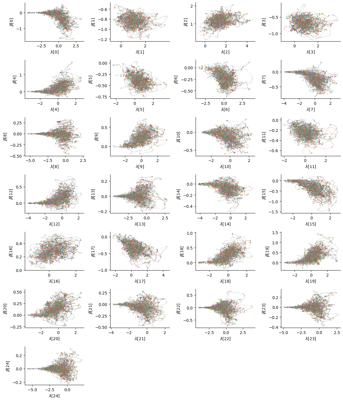
While some parameters (for instance the 15th) exhibit no particular correlations, the funnel geometry can still be observed for a few of them (4th, 13th, etc.). Ideally one would adopt a centered parametrization for those parameters to get a better approximation to the true posterior distribution, but here we also assess the ability of the sampler to explore these funnel geometries.
We can convince ourselves that the Horseshoe prior induces sparsity on the regression coefficients by looking at their posterior distribution:
_, axes = plt.subplots(n_row, n_col, sharex=True, figsize=(n_col * 3, n_row * 2))
axes = axes.flatten()
for i in range(n_pred):
    ax = axes[i]
    ax.hist(samples.position["beta"][..., i],
            bins=50, density=True, histtype="step")
    ax.set_xlabel(rf"$\beta$[{i}]")
    ax.get_yaxis().set_visible(False)
    ax.spines["left"].set_visible(False)
ax.set_xlim([-2, 2])
for j in range(i+1, n_col*n_row):
    axes[j].remove()
plt.tight_layout();
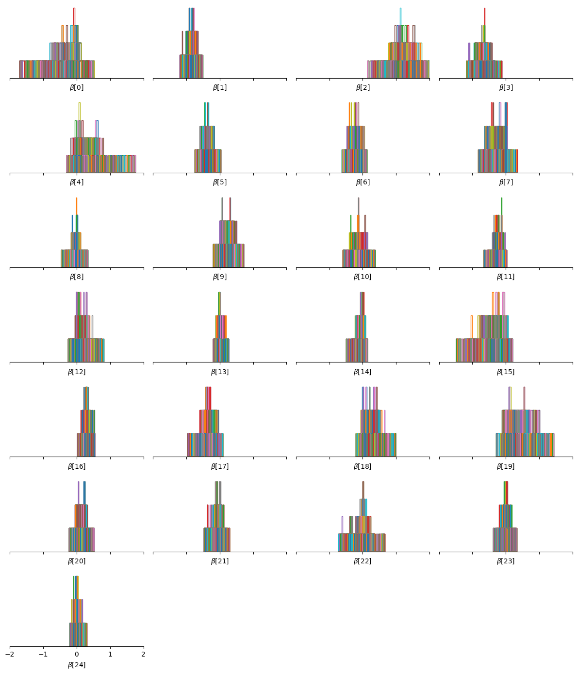
Indeed, many of the parameters are centered around \(0\).
Note
It is interesting to notice that the interactions for the parameters with large values do not exhibit funnel geometries.
Bibliography#
Carlos M Carvalho, Nicholas G Polson, and James G Scott. The horseshoe estimator for sparse signals. Biometrika, 97(2):465–480, 2010.
Dheeru Dua and Casey Graff. UCI machine learning repository. 2017. URL: http://archive.ics.uci.edu/ml.
Matthew D Hoffman and Pavel Sountsov. Tuning-free generalized hamiltonian monte carlo. In International Conference on Artificial Intelligence and Statistics, 7799–7813. PMLR, 2022.