Pathfinder

Pathfinder#

In this notebook we introduce the pathfinder [ZCGV22] algorithm and we show how to use it as a variational inference method or as an initialization tool for MCMC kernels.

import jax

from datetime import date
rng_key = jax.random.key(int(date.today().strftime("%Y%m%d")))

from matplotlib.patches import Ellipse
from sklearn.datasets import make_biclusters
import numpy as np

import jax.numpy as jnp
import blackjax

The Data#

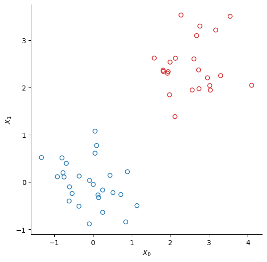
We create two clusters of points using scikit-learn’s make_bicluster function.

num_points = 50
X, rows, cols = make_biclusters(
    (num_points, 2), 2, noise=0.6, random_state=314, minval=-3, maxval=3
)
y = rows[0] * 1.0  # y[i] = whether point i belongs to cluster 1

../_images/fa97a3df3acdf2be30124c4c8391fb08183e1cffa2881be8b0cec259886842f8.png

The Model#

We use a simple logistic regression model to infer to which cluster each of the points belongs. We note \(y\) a binary variable that indicates whether a point belongs to the first cluster:

\[ y \sim \operatorname{Bernoulli}(p) \]

The probability \(p\) to belong to the first cluster commes from a logistic regression:

\[ p = \operatorname{logistic}(\Phi\,\boldsymbol{w}) \]

where \(w\) is a vector of weights whose priors are a normal prior centered on 0:

\[ \boldsymbol{w} \sim \operatorname{Normal}(0, \sigma) \]

And \(\Phi\) is the matrix that contains the data, so each row \(\Phi_{i,:}\) is the vector \(\left[X_0^i, X_1^i\right]\)

Phi = X
N, M = Phi.shape


def sigmoid(z):
    return jnp.exp(z) / (1 + jnp.exp(z))


def log_sigmoid(z):
    return z - jnp.log(1 + jnp.exp(z))


def logdensity_fn(w, alpha=1.0):
    """The log-probability density function of the posterior distribution of the model."""
    log_an = log_sigmoid(Phi @ w)
    an = Phi @ w
    log_likelihood_term = y * log_an + (1 - y) * jnp.log(1 - sigmoid(an))
    prior_term = alpha * w @ w / 2

    return -prior_term + log_likelihood_term.sum()

Pathfinder: Parallel Quasi-Newton Variational Inference#

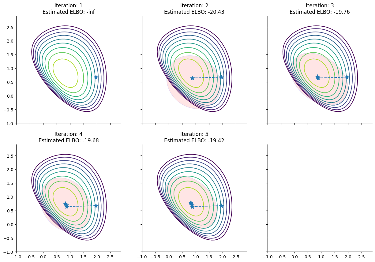
Starting from a random initialization, Pathfinder locates normal approximations to the target density along a quasi-Newton optimization path, with local covariance estimated using the inverse Hessian estimates produced by the optimizer. Pathfinder returns draws from the approximation with the lowest estimated Kullback-Leibler (KL) divergence to the true posterior. The optimizer is the limited memory BFGS algorithm.

To help understand the approximations that pathfinder evaluates during its run, here we plot for each step of the L-BFGS optimizer the approximation of the posterior distribution of the model derived by pathfinder and its ELBO:

# jaxopt lbfgs could fail, hack to keep trying util it works
stop = 0
while stop == 0:
    rng_key, init_key, infer_key = jax.random.split(rng_key, 3)
    w0 = jax.random.multivariate_normal(init_key, 2.0 + jnp.zeros(M), jnp.eye(M))
    _, info = blackjax.vi.pathfinder.approximate(infer_key, logdensity_fn, w0, ftol=1e-6)
    path = info.path
    stop = np.isfinite(path.elbo).mean()

WARNING: jaxopt.ZoomLineSearch: Linesearch failed, no stepsize satisfying sufficient decrease found.
INFO: jaxopt.ZoomLineSearch: Iter: 1000, Stepsize: 0.0, Decrease error: inf, Curvature error: inf
WARNING: jaxopt.ZoomLineSearch: The linesearch failed because the provided direction is not a descent direction. The slope (=nan) at stepsize=0 should be negative
WARNING: jaxopt.ZoomLineSearch: Cannot even make a step without getting Inf or Nan. The linesearch won't make a step and the optimizer is stuck.

WARNING: jaxopt.ZoomLineSearch: Linesearch failed, no stepsize satisfying sufficient decrease found.
INFO: jaxopt.ZoomLineSearch: Iter: 1000, Stepsize: 0.0, Decrease error: inf, Curvature error: inf
WARNING: jaxopt.ZoomLineSearch: The linesearch failed because the provided direction is not a descent direction. The slope (=nan) at stepsize=0 should be negative
WARNING: jaxopt.ZoomLineSearch: Cannot even make a step without getting Inf or Nan. The linesearch won't make a step and the optimizer is stuck.

../_images/214e34de2ffda65ca1735137487a8e0bca1a679ab5e3751612b3451a3acb57fe.png

Pathfinder as a Variational Inference Method#

Pathfinder can be used as a variational inference method. We first create a pathfinder object pf which contains two functions approximate and sample:

pf = blackjax.pathfinder(logdensity_fn)
rng_key, approx_key = jax.random.split(rng_key)
state, _ = pf.approximate(approx_key, w0, ftol=1e-4)

We can now get samples from the approximation:

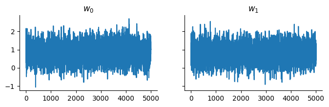
rng_key, sample_key = jax.random.split(rng_key)
samples, _ = pf.sample(sample_key, state, 5_000)

And display the trace:

../_images/396a8e0089684feafd7cb7c5ffd5a8f8161a73b330ec6abfa4fb244fbc6816fa.png

Please note that pathfinder is implemented as follows:

it runs L-BFGS optimization and finds the best approximation in the init phase
step phase it’s just sampling from a multinormal distribution, whose parameters have been already estimated

Hence it makes sense to jit the init function and then use the sample helper function in the pathfinder object instead of implementing the inference loop:

%%time

state, _ = jax.jit(pf.approximate)(approx_key, w0)
samples, _ = pf.sample(sample_key, state, 5_000)

CPU times: user 3.12 s, sys: 23.5 ms, total: 3.14 s
Wall time: 3.1 s

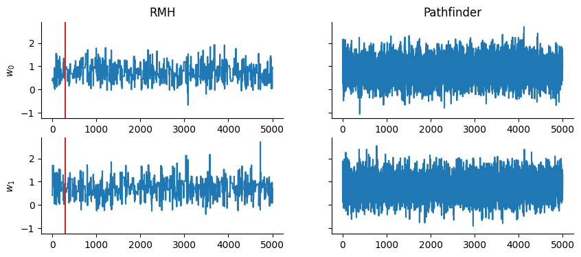
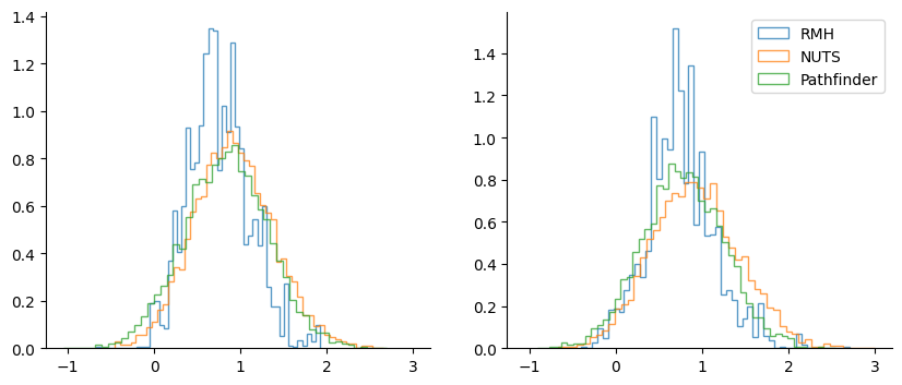
Quick comparison against the Rosenbluth-Metropolis-Hastings kernel rmh:

def inference_loop(rng_key, kernel, initial_state, num_samples):
    @jax.jit
    def one_step(state, rng_key):
        state, info = kernel(rng_key, state)
        return state, (state, info)

    keys = jax.random.split(rng_key, num_samples)
    return jax.lax.scan(one_step, initial_state, keys)


rmh = blackjax.rmh(
    logdensity_fn, blackjax.mcmc.random_walk.normal(sigma=jnp.ones(M) * 0.7)
)
state_rmh = rmh.init(w0)
rng_key, sample_key = jax.random.split(rng_key)
_, (samples_rmh, _) = inference_loop(sample_key, rmh.step, state_rmh, 5_000)

../_images/1c9dfd20b0cd9ba9f4b028ecd398c3db448dbc70277a86d78cfa8d6a7504faa8.png

Pathfinder as an Initialization Tool for MCMC Kernels#

Pathfinder uses internally the inverse hessian estimation of the L-BFGS optimizer to evaluate the approximations to the target distribution along the quasi-Newton optimization path.

We can calculate explicitly this inverse hessian matrix for a step of the optimization path using the blackjax.optimizers.lbfgs.lbfgs_inverse_hessian_formula_1 function:

from blackjax.optimizers.lbfgs import lbfgs_inverse_hessian_formula_1

inverse_mass_matrix = lbfgs_inverse_hessian_formula_1(
    state.alpha, state.beta, state.gamma
)
inverse_mass_matrix

Array([[ 0.1482668 , -0.0374889 ],
       [-0.03748889,  0.20744953]], dtype=float32)

This estimation of the inverse mass matrix, coupled with Nesterov’s dual averaging adaptation for estimating the step size, yields an alternative adaptation scheme for initializing MCMC kernels.

This scheme is implemented in blackjax.pathfinder_adaptation function:

adapt = blackjax.pathfinder_adaptation(blackjax.nuts, logdensity_fn)
rng_key, sample_key = jax.random.split(rng_key)
(state, parameters), info = adapt.run(sample_key, w0, 400)

nuts = blackjax.nuts(logdensity_fn, **parameters)
init0 = nuts.init(state.position)
rng_key, sample_key = jax.random.split(rng_key)
_, (samples_nuts, _) = inference_loop(sample_key, nuts.step, init0, 5000)

../_images/5a899f787e12356bb1e0497803991e1b2ec65f5c80fc3a10bb53dbba8eb5c124.png

Some Caveats#

L-BFGS algorithm struggles with float32s and log-likelihood functions; it’s suggested to use double precision numbers. In order to do that in jax a configuration variable needs to be set up at initialization time (see here)
Otherwise you can stick with float32 mode and try to tweak ftol, gtol, or the initialization point
It may make sense to start pathfinder with a “bad” initialization point, in order to make the L-BFGS algorithm run longer and have more datapoints to estimate the inverse hessian matrix.

[ZCGV22]

Lu Zhang, Bob Carpenter, Andrew Gelman, and Aki Vehtari. Pathfinder: parallel quasi-newton variational inference. 2022. arXiv:2108.03782.